Munson B.R. Fundamentals of Fluid Mechanics

Подождите немного. Документ загружается.

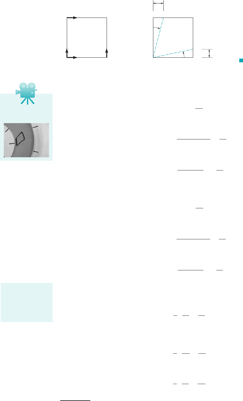
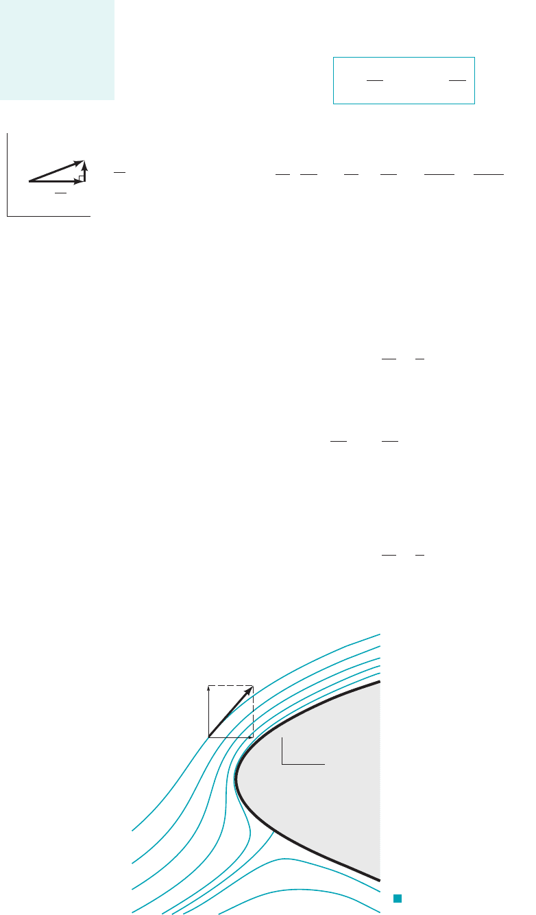
rotate through the angles and to the new positions and , as is shown in Fig. 6.4b.

The angular velocity of line OA, is

For small angles

(6.10)

so that

Note that if is positive, will be counterclockwise. Similarly, the angular velocity of the

line OB is

and

(6.11)

so that

In this instance if is positive, will be clockwise. The rotation, of the element about the

z axis is defined as the average of the angular velocities and of the two mutually perpendicular

lines OA and OB.

Thus, if counterclockwise rotation is considered to be positive, it follows that

(6.12)

Rotation of the field element about the other two coordinate axes can be obtained in a similar

manner with the result that for rotation about the x axis

(6.13)

and for rotation about the y axis

(6.14)v

⫽

⫺

⫽

⫺

⫽

⫺

Ⲑ

⫽ lim

dtS0

10u

Ⲑ

0y2 dt

d⫽

tan db ⬇ db ⫽

10u

Ⲑ

0y2 dy dt

⫽

⫽ lim

dtS0

Ⲑ

⫽ lim

dtS0

10v

Ⲑ

0x2 dt

d⫽

tan da ⬇ da ⫽

10v

Ⲑ

0x2 dx dt

⫽

⫽ lim

dtS0

OB¿OA¿dbda

6.1 Fluid Element Kinematics 267

Rotation of fluid

particles is related

to certain velocity

gradients in the

flow field.

)

δβ

δα

(a)(b)

∂

u + y

___

∂

v + x

___

∂

F I G U R E 6.4

Angular motion and deforma-

tion of a fluid element.

With this definition can also be interpreted to be the angular velocity of the bisector of the angle between the lines OA and OB.v

V6.3 Shear

deformation

JWCL068_ch06_263-331.qxd 9/23/08 12:17 PM Page 267

The three components, and can be combined to give the rotation vector, in the form

(6.15)

An examination of this result reveals that is equal to one-half the curl of the velocity vector. That is,

(6.16)

since by definition of the vector operator

The vorticity, is defined as a vector that is twice the rotation vector; that is,

(6.17)

The use of the vorticity to describe the rotational characteristics of the fluid simply eliminates the

factor associated with the rotation vector. The figure in the margin shows vorticity contours of

the wing tip vortex flow shortly after an aircraft has passed. The lighter colors indicate stronger

vorticity. (See also Fig. 4.3.)

We observe from Eq. 6.12 that the fluid element will rotate about the z axis as an undeformed

block only when Otherwise the rotation will be associated

with an angular deformation. We also note from Eq. 6.12 that when the rotation

around the z axis is zero. More generally if then the rotation 1and the vorticity2are zero,

and flow fields for which this condition applies are termed irrotational. We will find in Section 6.4

that the condition of irrotationality often greatly simplifies the analysis of complex flow fields.

However, it is probably not immediately obvious why some flow fields would be irrotational, and we

will need to examine this concept more fully in Section 6.4.

⵱ⴛV ⫽ 0,

Ⲑ

0y ⫽ 0v

Ⲑ

0y ⫽⫺0v

Ⲑ

0x.1i.e., v

⫽⫺v

Z ⫽ 2 ␻ ⫽ ⵱ⴛV

⫽

⫺

b i

⫹

⫺

b j

⫹

⫺

b k

⵱ⴛV ⫽

∞

⵱ⴛV

␻ ⫽

curl V ⫽

⵱ⴛV

␻

␻ ⫽ v

⫹ v

␻,v

, v

268 Chapter 6 ■ Differential Analysis of Fluid Flow

Wing

Vorticity in a flow

field is related to

fluid particle rota-

tion.

GIVEN For a certain two-dimensional flow field the velocity

is given by the equation

V ⫽ 1x

⫺ y

⫺ 2xyj

FIND Is this flow irrotational?

OLUTION

Vorticity

zero, since by definition of two-dimensional flow u and are not

functions of z, and w is zero. In this instance the condition for ir-

rotationality simply becomes or

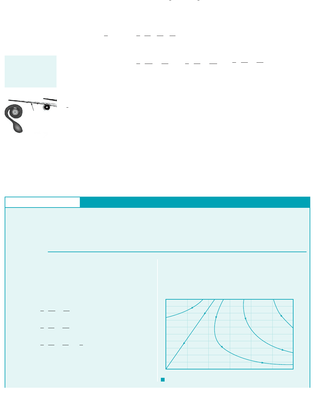
The streamlines for the steady, two-dimensional flow of this ex-

ample are shown in Fig. E6.1. (Information about how to calculate

Ⲑ

0x ⫽ 0u

Ⲑ

0y.

⫽ 0

XAMPLE 6.1

For an irrotational flow the rotation vector, having the compo-

nents given by Eqs. 6.12, 6.13, and 6.14 must be zero. For the pre-

scribed velocity field

and therefore

Thus, the flow is irrotational.

(Ans)

COMMENTS It is to be noted that for a two-dimensional flow

field 1where the flow is in the x–y plane2 and will always be

⫽

⫺

b⫽

31⫺2y2⫺ 1⫺2y24⫽ 0

⫽

⫺

b⫽ 0

⫽

⫺

b⫽ 0

u ⫽ x

⫺ y

v ⫽⫺2xy

w ⫽ 0

␻,

F I G U R E E6.1

JWCL068_ch06_263-331.qxd 9/23/08 12:17 PM Page 268

In addition to the rotation associated with the derivatives and it is observed

from Fig. 6.4b that these derivatives can cause the fluid element to undergo an angular

deformation, which results in a change in shape of the element. The change in the original right

angle formed by the lines OA and OB is termed the shearing strain, and from Fig. 6.4b

where is considered to be positive if the original right angle is decreasing. The rate of change

of is called the rate of shearing strain or the rate of angular deformation and is commonly

denoted with the symbol The angles and are related to the velocity gradients through Eqs.

6.10 and 6.11 so that

and, therefore,

(6.18)

As we will learn in Section 6.8, the rate of angular deformation is related to a corresponding shearing

stress which causes the fluid element to change in shape. From Eq. 6.18 we note that if

the rate of angular deformation is zero, and this condition corresponds to the case

in which the element is simply rotating as an undeformed block 1Eq. 6.122. In the remainder of this

chapter we will see how the various kinematical relationships developed in this section play an important

role in the development and subsequent analysis of the differential equations that govern fluid motion.

Ⲑ

0y ⫽⫺0v

Ⲑ

0x,

᝽

⫽

⫹

᝽

⫽ lim

dtS0

⫽ lim

dtS0

10v

Ⲑ

0x2 dt ⫹ 10u

Ⲑ

0y2 dt

dbdag

᝽

dg ⫽ da ⫹ db

dg,

Ⲑ

0x,0u

Ⲑ

6.2 Conservation of Mass 269

As is discussed in Section 5.1, conservation of mass requires that the mass, M, of a system remain

constant as the system moves through the flow field. In equation form this principle is expressed as

We found it convenient to use the control volume approach for fluid flow problems, with the control

volume representation of the conservation of mass written as

(6.19)

where the equation 1commonly called the continuity equation2can be applied to a finite control

volume 1cv2, which is bounded by a control surface 1cs2. The first integral on the left side of Eq. 6.19

represents the rate at which the mass within the control volume is changing, and the second integral

represents the net rate at which mass is flowing out through the control surface 1rate of mass

outflow rate of mass inflow2. To obtain the differential form of the continuity equation, Eq. 6.19

is applied to an infinitesimal control volume.

6.2.1 Differential Form of Continuity Equation

We will take as our control volume the small, stationary cubical element shown in Fig. 6.5a. At

the center of the element the fluid density is and the velocity has components u, and w. Since

the element is small, the volume integral in Eq. 6.19 can be expressed as

(6.20)

冮

r dV⫺ ⬇

dx dy dz

v,r

⫺

冮

dV⫺⫹

冮

V ⴢ nˆ dA ⫽ 0

sys

⫽ 0

6.2 Conservation of Mass

Conservation of

mass requires that

the mass of a

system remain

constant.

streamlines for a given velocity field is given in Sections 4.1.4

and 6.2.3.) It is noted that all of the streamlines (except for the one

through the origin) are curved. However, because the flow is irro-

tational, there is no rotation of the fluid elements. That is, lines

OA and OB of Fig. 6.4 rotate with the same speed but in opposite

directions.

AsshownbyEq.6.17,theconditionofirrotationalityisequivalent

tothefactthatthevorticity, ,iszeroorthecurlofthevelocityiszero.Z

JWCL068_ch06_263-331.qxd 9/23/08 12:17 PM Page 269

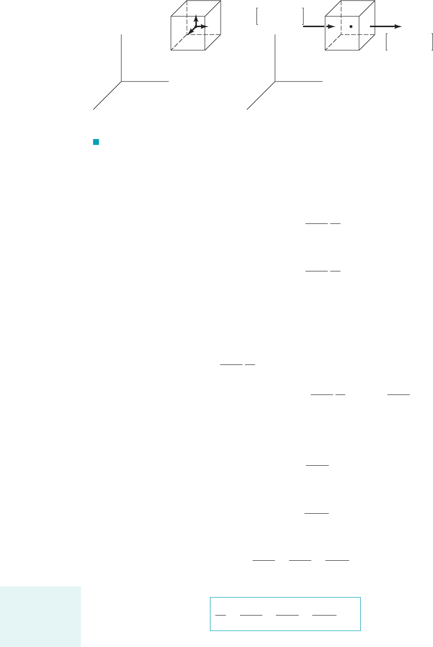
The rate of mass flow through the surfaces of the element can be obtained by considering the flow

in each of the coordinate directions separately. For example, in Fig. 6.5b flow in the x direction is

depicted. If we let represent the x component of the mass rate of flow per unit area at the center

of the element, then on the right face

(6.21)

and on the left face

(6.22)

Note that we are really using a Taylor series expansion of and neglecting higher order terms

such as and so on. When the right-hand sides of Eqs. 6.21 and 6.22 are multiplied by

the area the rate at which mass is crossing the right and left sides of the element are obtained

as is illustrated in Fig. 6.5b. When these two expressions are combined, the net rate of mass flowing

from the element through the two surfaces can be expressed as

(6.23)

For simplicity, only flow in the x direction has been considered in Fig. 6.5b, but, in general,

there will also be flow in the y and z directions. An analysis similar to the one used for flow in the

x direction shows that

(6.24)

and

(6.25)

Thus,

(6.26)

From Eqs. 6.19, 6.20, and 6.26 it now follows that the differential equation for conservation of mass is

(6.27)

As previously mentioned, this equation is also commonly referred to as the continuity equation.

⫹

01ru2

⫹

01rv2

⫹

01rw2

⫽ 0

Net rate of

mass outflow

⫽ c

01ru2

⫹

01rv2

⫹

01rw2

d dx dy dz

Net rate of mass

outflow in z direction

⫽

01rw2

dx dy dz

Net rate of mass

outflow in y direction

⫽

01rv2

dx dy dz

⫺ cru ⫺

01ru2

d dy dz ⫽

01ru2

dx dy dz

Net rate of mass

outflow in x direction

⫽ cru ⫹

01ru2

d dy dz

dy dz,

1dx2

, 1dx2

ru0

x⫺1dx

Ⲑ

⫽ ru ⫺

01ru2

ru0

x⫹1dx

Ⲑ

⫽ ru ⫹

01ru2

The continuity

equation is one of

the fundamental

equations of fluid

mechanics.

270 Chapter 6 ■ Differential Analysis of Fluid Flow

u –

(

)

y z

_____

∂

δδρ

(a)(b)

u +

(

)

y z

_____

∂

δδρ

F I G U R E 6.5 A differential element for the development of conservation of mass equation.

JWCL068_ch06_263-331.qxd 9/23/08 12:17 PM Page 270

The continuity equation is one of the fundamental equations of fluid mechanics and, as

expressed in Eq. 6.27, is valid for steady or unsteady flow, and compressible or incompressible

fluids. In vector notation, Eq. 6.27 can be written as

(6.28)

Two special cases are of particular interest. For steady flow of compressible fluids

(6.29)

This follows since by definition is not a function of time for steady flow, but could be a function

of position. For incompressible fluids the fluid density, is a constant throughout the flow field

so that Eq. 6.28 becomes

(6.30)

(6.31)

Equation 6.31 applies to both steady and unsteady flow of incompressible fluids. Note that Eq. 6.31

is the same as that obtained by setting the volumetric dilatation rate 1Eq. 6.92equal to zero. This

result should not be surprising since both relationships are based on conservation of mass for

incompressible fluids. However, the expression for the volumetric dilatation rate was developed

from a system approach, whereas Eq. 6.31 was developed from a control volume approach. In the

former case the deformation of a particular differential mass of fluid was studied, and in the latter

case mass flow through a fixed differential volume was studied.

⫹

⫽ 0

⵱ⴢV ⫽ 0

01ru2

⫹

01rv2

⫹

01rw2

⫽ 0

⵱ⴢrV ⫽ 0

⫹ ⵱ⴢrV ⫽ 0

6.2 Conservation of Mass 271

For incompressible

fluids the continuity

equation reduces to

a simple relation-

ship involving cer-

tain velocity gradi-

ents.

GIVEN The velocity components for a certain incompress-

ible, steady flow field are

w ⫽ ?

v ⫽ xy ⫹ yz ⫹ z

u ⫽ x

⫹ y

⫹ z

FIND Determine the form of the z component, w, required to

satisfy the continuity equation.

Continuity Equation

XAMPLE 6.2

OLUTION

so that the required expression for is

Integration with respect to z yields

(Ans)

COMMENT The third velocity component cannot be explic-

itly determined since the function can have any form and

conservation of mass will still be satisfied. The specific form of

this function will be governed by the flow field described by these

velocity components—that is, some additional information is

needed to completely determine w.

f1x, y2

w ⫽⫺3xz ⫺

⫹ f1x, y2

⫽⫺2x ⫺ 1x ⫹ z2⫽⫺3x ⫺ z

Ⲑ

Any physically possible velocity distribution must for an incom-

pressible fluid satisfy conservation of mass as expressed by the

continuity equation

For the given velocity distribution

⫽ 2x

and

⫽ x ⫹ z

⫹

⫽ 0

JWCL068_ch06_263-331.qxd 9/23/08 12:17 PM Page 271

6.2.2 Cylindrical Polar Coordinates

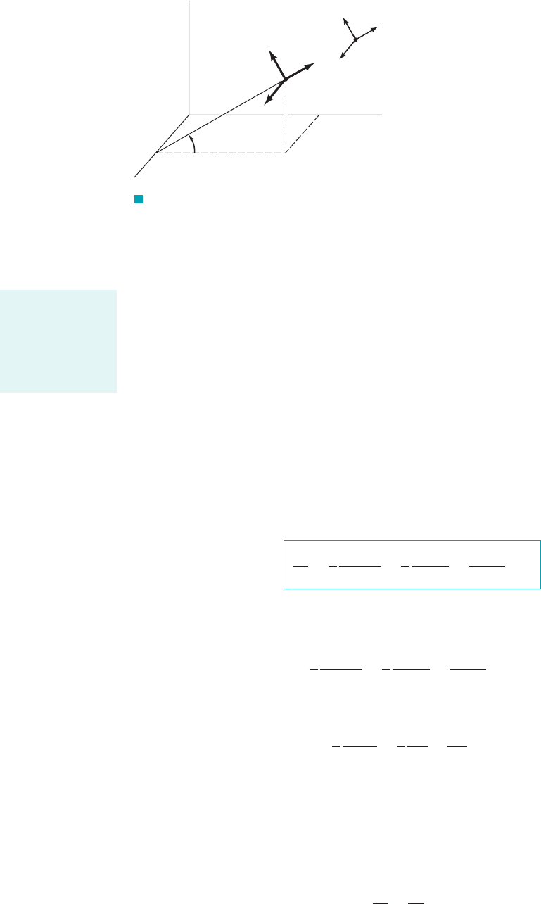
For some problems it is more convenient to express the various differential relationships in cylindrical

polar coordinates rather than Cartesian coordinates. As is shown in Fig. 6.6, with cylindrical coordinates

a point is located by specifying the coordinates r, and z. The coordinate r is the radial distance from

the z axis, is the angle measured from a line parallel to the x axis 1with counterclockwise taken as

positive2, and z is the coordinate along the z axis. The velocity components, as sketched in Fig. 6.6,

are the radial velocity, the tangential velocity, and the axial velocity, Thus, the velocity at

some arbitrary point P can be expressed as

(6.32)

where and are the unit vectors in the r, and z directions, respectively, as are illustrated

in Fig. 6.6. The use of cylindrical coordinates is particularly convenient when the boundaries of

the flow system are cylindrical. Several examples illustrating the use of cylindrical coordinates will

be given in succeeding sections in this chapter.

The differential form of the continuity equation in cylindrical coordinates is

(6.33)

This equation can be derived by following the same procedure used in the preceding section 1see

Problem 6.202. For steady, compressible flow

(6.34)

For incompressible fluids 1for steady or unsteady flow2

(6.35)

6.2.3 The Stream Function

Steady, incompressible, plane, two-dimensional flow represents one of the simplest types of flow

of practical importance. By plane, two-dimensional flow we mean that there are only two velocity

components, such as u and when the flow is considered to be in the x–y plane. For this flow

the continuity equation, Eq. 6.31, reduces to

(6.36)

⫹

⫽ 0

01rv

⫹

⫽ 0

01rrv

⫹

01rv

⫹

01rv

⫽ 0

⫹

01rrv

⫹

01rv

⫹

01rv

⫽ 0

u,ê

, ê

V ⫽ v

⫹ v

272 Chapter 6 ■ Differential Analysis of Fluid Flow

F I G U R E 6.6 The representation of

velocity components in cylindrical polar coordinates.

For some problems,

velocity components

expressed in cylin-

drical polar coordi-

nates will be

convenient.

JWCL068_ch06_263-331.qxd 9/23/08 12:17 PM Page 272

We still have two variables, u and to deal with, but they must be related in a special way as

indicated by Eq. 6.36. This equation suggests that if we define a function called the stream

function, which relates the velocities shown by the figure in the margin as

(6.37)

then the continuity equation is identically satisfied. This conclusion can be verified by simply

substituting the expressions for u and into Eq. 6.36 so that

Thus, whenever the velocity components are defined in terms of the stream function we know that

conservation of mass will be satisfied. Of course, we still do not know what is for a particular

problem, but at least we have simplified the analysis by having to determine only one unknown

function, rather than the two functions, and

Another particular advantage of using the stream function is related to the fact that lines

along which is constant are streamlines. Recall from Section 4.1.4 that streamlines are lines in

the flow field that are everywhere tangent to the velocities, as is illustrated in Fig. 6.7. It follows

from the definition of the streamline that the slope at any point along a streamline is given by

The change in the value of as we move from one point to a nearby point

is given by the relationship:

Along a line of constant we have so that

and, therefore, along a line of constant

which is the defining equation for a streamline. Thus, if we know the function we can plot

lines of constant to provide the family of streamlines that are helpful in visualizing the patternc

c1x, y2

⫽

⫺v dx ⫹ u dy ⫽ 0

dc ⫽ 0c

dc ⫽

dx ⫹

dy ⫽⫺v dx ⫹ u dy

y ⫹ dy21x ⫹ dx,1x, y2c

⫽

v1x, y2.u1x, y2c1x, y2,

c1x, y2

b⫹

a⫺

b⫽

0x 0y

⫺

0y 0x

⫽ 0

u ⫽

v ⫽⫺

c1x, y2,

6.2 Conservation of Mass 273

Velocity compo-

nents in a two-

dimensional flow

field can be ex-

pressed in terms of

a stream function.

u =

∂

v = –

∂

F I G U R E 6.7 Velocity and velocity

components along a streamline.

Streamlines

JWCL068_ch06_263-331.qxd 9/23/08 12:17 PM Page 273

of flow. There are an infinite number of streamlines that make up a particular flow field, since for

each constant value assigned to a streamline can be drawn.

The actual numerical value associated with a particular streamline is not of particular

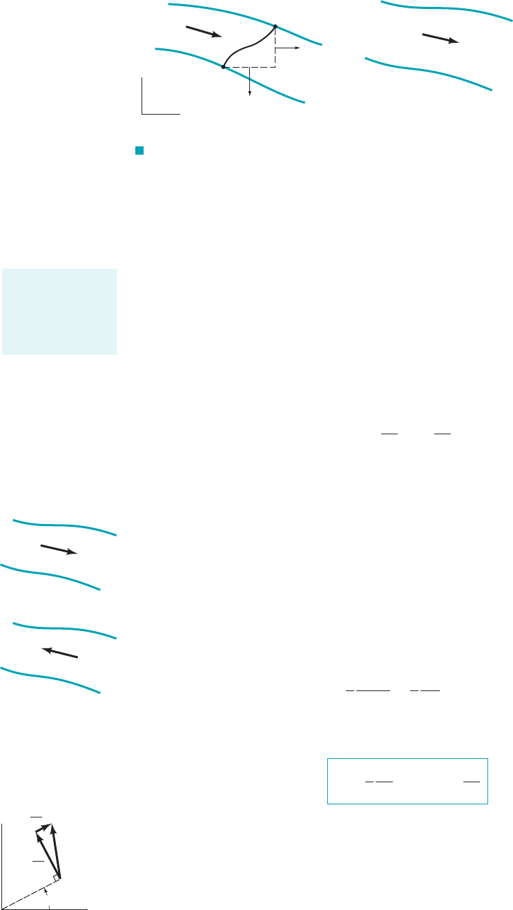
significance, but the change in the value of is related to the volume rate of flow. Consider two

closely spaced streamlines, shown in Fig. 6.8a. The lower streamline is designated and the upper

one Let dq represent the volume rate of flow 1per unit width perpendicular to the x–y

plane2passing between the two streamlines. Note that flow never crosses streamlines, since by

definition the velocity is tangent to the streamline. From conservation of mass we know that the

inflow, dq, crossing the arbitrary surface AC of Fig. 6.8a must equal the net outflow through surfaces

AB and BC. Thus,

or in terms of the stream function

(6.38)

The right-hand side of Eq. 6.38 is equal to so that

(6.39)

Thus, the volume rate of flow, q, between two streamlines such as and of Fig. 6.8b can be

determined by integrating Eq. 6.39 to yield

(6.40)

The relative value of with respect to determines the direction of flow, as shown by the figure

in the margin.

In cylindrical coordinates the continuity equation 1Eq. 6.352for incompressible, plane, two-

dimensional flow reduces to

(6.41)

and the velocity components, and can be related to the stream function, through the

equations

(6.42)

as shown by the figure in the margin.

Substitution of these expressions for the velocity components into Eq. 6.41 shows that the

continuity equation is identically satisfied. The stream function concept can be extended to

axisymmetric flows, such as flow in pipes or flow around bodies of revolution, and to two-

dimensional compressible flows. However, the concept is not applicable to general three-dimensional

flows.

⫽

⫽⫺

c1r, u2,v

01rv

⫹

⫽ 0

q ⫽

冮

dc ⫽ c

⫺ c

dq ⫽ dc

dq ⫽

dy ⫹

dq ⫽ u dy ⫺ v dx

c ⫹ dc.

274 Chapter 6 ■ Differential Analysis of Fluid Flow

+ d

ψψ

u dy

– v dx

(b)(a)

F I G U R E 6.8 The flow between two streamlines.

The change in the

value of the stream

function is related

to the volume rate

of flow.

= –

∂

JWCL068_ch06_263-331.qxd 9/23/08 12:17 PM Page 274

6.3 Conservation of Linear Momentum 275

GIVEN The velocity components in a steady, incompressible,

two-dimensional flow field are

v ⫽ 4x

u ⫽ 2y

FIND

(a) Determine the corresponding stream function and

(b) Show on a sketch several streamlines. Indicate the direction

of flow along the streamlines.

OLUTION

Stream Function

Other streamlines can be obtained by setting equal to various

constants. It follows from Eq. 1 that the equations of these stream-

lines can be expressed in the form

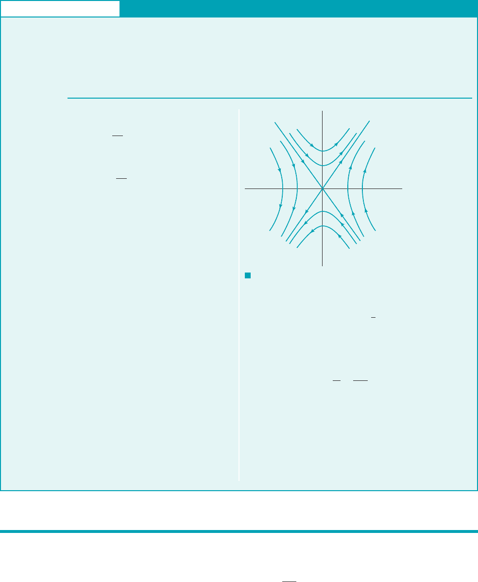
which we recognize as the equation of a hyperbola. Thus, the

streamlines are a family of hyperbolas with the stream-

lines as asymptotes. Several of the streamlines are plotted in

Fig. E6.3. Since the velocities can be calculated at any point, the

direction of flow along a given streamline can be easily de-

duced. For example, so that if

and if The direction of flow is indicated on the

figure.

x 6 0.v 6 0

x 7 0v 7 0

v ⫽⫺0c

Ⲑ

0x ⫽ 4x

c ⫽ 0

⫺

Ⲑ

⫽ 1

1for c ⫽ 02

y ⫽⫾12

XAMPLE 6.3

(a) From the definition of the stream function 1Eqs. 6.372

and

The first of these equations can be integrated to give

where is an arbitrary function of x. Similarly from the sec-

ond equation

where is an arbitrary function of y. It now follows that in or-

der to satisfy both expressions for the stream function

(Ans)

where C is an arbitrary constant.

COMMENT Since the velocities are related to the derivatives

of the stream function, an arbitrary constant can always be added

to the function, and the value of the constant is actually of no con-

sequence. Usually, for simplicity, we set so that for this

particular example the simplest form for the stream function is

(1) (Ans)

Either answer indicated would be acceptable.

(b) Streamlines can now be determined by setting

and plotting the resulting curve. With the above expression for

the value of at the origin is zero so that the

equation of the streamline passing through the origin 1the

streamline2is

0 ⫽⫺2x

⫹ y

c ⫽ 0

cc 1with C ⫽ 02

c ⫽ constant

c ⫽⫺2x

⫹ y

C ⫽ 0

c ⫽⫺2x

⫹ y

⫹ C

1y2

c ⫽⫺2x

⫹ f

1y2

1x2

c ⫽ y

⫹ f

1x2

v ⫽⫺

⫽ 4x

u ⫽

⫽ 2y

= 0

F I G U R E E6.3

To develop the differential momentum equations we can start with the linear momentum

equation

(6.43)

where F is the resultant force acting on a fluid mass, P is the linear momentum defined as

P ⫽

冮

sys

V dm

F ⫽

sys

6.3 Conservation of Linear Momentum

JWCL068_ch06_263-331.qxd 9/23/08 12:17 PM Page 275

276 Chapter 6 ■ Differential Analysis of Fluid Flow

and the operator is the material derivative 1see Section 4.2.122. In the last chapter it was

demonstrated how Eq. 6.43 in the form

(6.44)

could be applied to a finite control volume to solve a variety of flow problems. To obtain the

differential form of the linear momentum equation, we can either apply Eq. 6.43 to a differential

system, consisting of a mass, or apply Eq. 6.44 to an infinitesimal control volume, which

initially bounds the mass It is probably simpler to use the system approach since application

of Eq. 6.43 to the differential mass, yields

where is the resultant force acting on Using this system approach can be treated as a

constant so that

But is the acceleration, a, of the element. Thus,

(6.45)

which is simply Newton’s second law applied to the mass This is the same result that would

be obtained by applying Eq. 6.44 to an infinitesimal control volume 1see Ref. 12. Before we can

proceed, it is necessary to examine how the force can be most conveniently expressed.

6.3.1 Description of Forces Acting on the Differential Element

In general, two types of forces need to be considered: surface forces, which act on the surface of the

differential element, and body forces, which are distributed throughout the element. For our purpose,

the only body force, of interest is the weight of the element, which can be expressed as

(6.46)

where g is the vector representation of the acceleration of gravity. In component form

(6.47a)

(6.47b)

(6.47c)

where and are the components of the acceleration of gravity vector in the x, y, and z

directions, respectively.

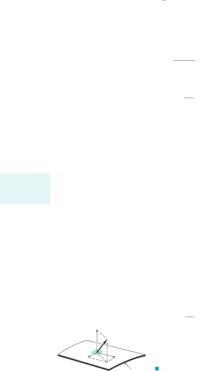
Surface forces act on the element as a result of its interaction with its surroundings. At any

arbitrary location within a fluid mass, the force acting on a small area, which lies in an arbitrary

surface, can be represented by as is shown in Fig. 6.9. In general, will be inclined with

respect to the surface. The force can be resolved into three components, and

where is normal to the area, , and and are parallel to the area and orthogonal to

each other. The normal stress, , is defined as

⫽ lim

dAS0

dAdF

,dF

, dF

,dF

dA,

, g

⫽ dm g

dF ⫽ dm a

Ⲑ

dF ⫽ dm

dmdm.dF

dF ⫽

D1V dm2

dm,

dm.

dV⫺,dm,

contents of the

control volume

⫽

冮

Vr dV⫺⫹

冮

VrV ⴢ nˆ dA

D12

Ⲑ

Both surface forces

and body forces

generally act on

fluid particles.

Arbitrary

surface

F I G U R E 6.9 Components of force acting

on an arbitrary differential area.

JWCL068_ch06_263-331.qxd 9/23/08 12:17 PM Page 276