Munson B.R. Fundamentals of Fluid Mechanics

Подождите немного. Документ загружается.

and the shearing stresses are defined as

and

We will use for normal stresses and for shearing stresses. The intensity of the force per unit

area at a point in a body can thus be characterized by a normal stress and two shearing stresses, if the

orientation of the area is specified. For purposes of analysis it is usually convenient to reference the

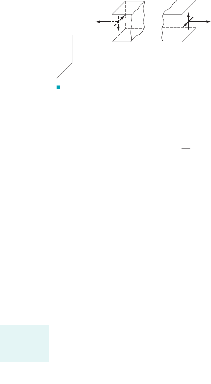
area to the coordinate system. For example, for the rectangular coordinate system shown in Fig. 6.10

we choose to consider the stresses acting on planes parallel to the coordinate planes. On the plane

ABCD of Fig. 6.10a, which is parallel to the y–zplane, the normal stress is denoted and the shearing

stresses are denoted as and To easily identify the particular stress component we use a double

subscript notation. The first subscript indicates the direction of the normal to the plane on which

the stress acts, and the second subscript indicates the direction of the stress. Thus, normal stresses have

repeated subscripts, whereas the subscripts for the shearing stresses are always different.

It is also necessary to establish a sign convention for the stresses. We define the positive direction

for the stress as the positive coordinate direction on the surfaces for which the outward normal is in

the positive coordinate direction. This is the case illustrated in Fig. 6.10a where the outward normal

to the area ABCD is in the positive x direction. The positive directions for and are as shown

in Fig. 6.10a. If the outward normal points in the negative coordinate direction, as in Fig. 6.10b for

the area then the stresses are considered positive if directed in the negative coordinate

directions. Thus, the stresses shown in Fig. 6.10b are considered to be positive when directed as shown.

Note that positive normal stresses are tensile stresses; that is, they tend to “stretch” the material.

It should be emphasized that the state of stress at a point in a material is not completely

defined by simply three components of a “stress vector.” This follows, since any particular stress

vector depends on the orientation of the plane passing through the point. However, it can be shown

that the normal and shearing stresses acting on any plane passing through a point can be expressed

in terms of the stresses acting on three orthogonal planes passing through the point 1Ref. 22.

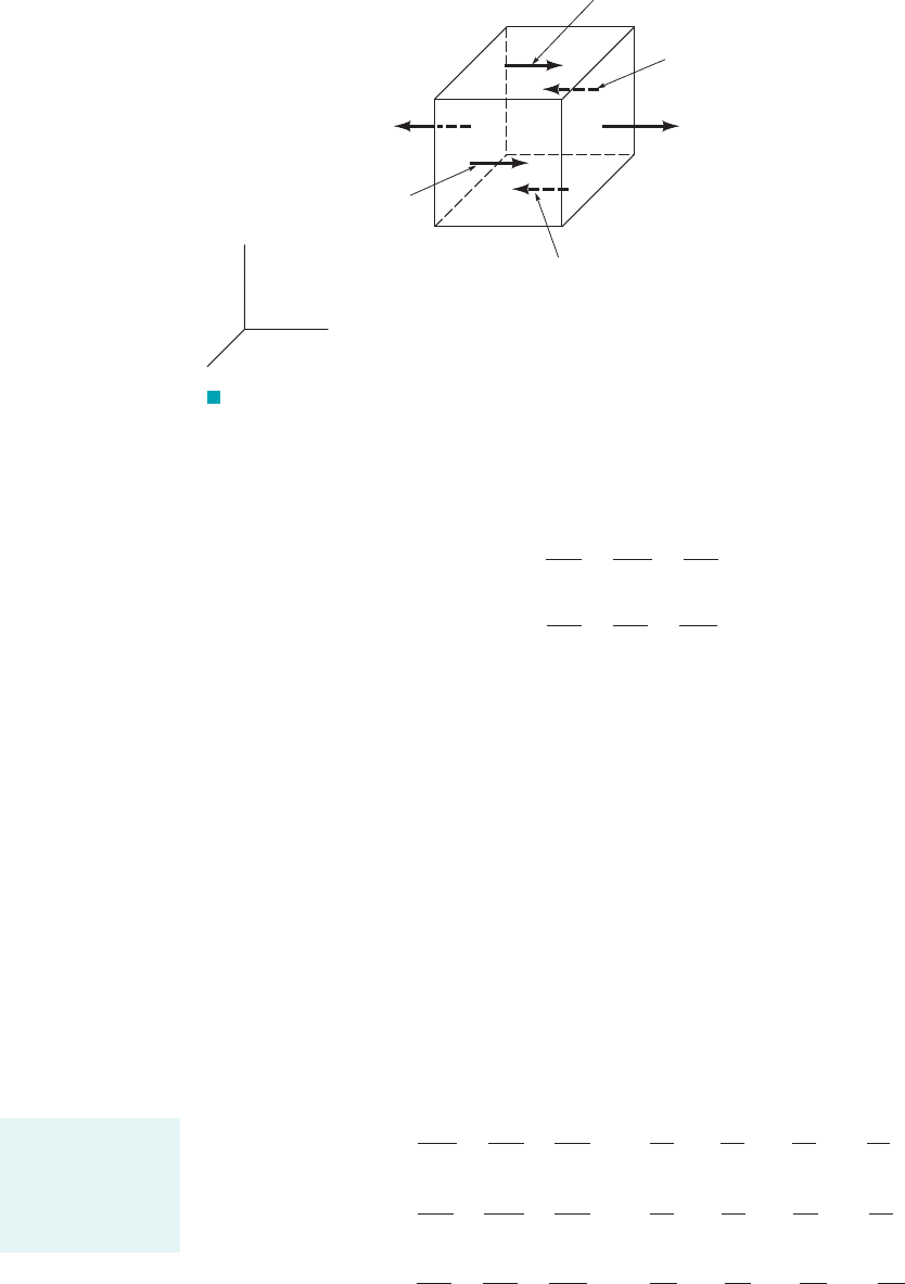
We now can express the surface forces acting on a small cubical element of fluid in terms

of the stresses acting on the faces of the element as shown in Fig. 6.11. It is expected that in general

the stresses will vary from point to point within the flow field. Thus, through the use of Taylor

series expansions we will express the stresses on the various faces in terms of the corresponding

stresses at the center of the element of Fig. 6.11 and their gradients in the coordinate directions.

For simplicity only the forces in the x direction are shown. Note that the stresses must be multiplied

by the area on which they act to obtain the force. Summing all these forces in the x direction yields

(6.48a)dF

⫽ a

⫹

b dx dy dz

A¿B¿C¿D¿,

⫽ lim

dAS0

⫽ lim

dAS0

6.3 Conservation of Linear Momentum 277

(b)(a)

F I G U R E 6.10 Double subscript notation for stresses.

Surface forces can

be expressed in

terms of the shear

and normal

stresses.

JWCL068_ch06_263-331.qxd 9/23/08 12:17 PM Page 277

for the resultant surface force in the x direction. In a similar manner the resultant surface forces in

the y and z directions can be obtained and expressed as

(6.48b)

(6.48c)

The resultant surface force can now be expressed as

(6.49)

and this force combined with the body force, yields the resultant force, acting on the

differential mass, That is,

6.3.2 Equations of Motion

The expressions for the body and surface forces can now be used in conjunction with Eq. 6.45 to

develop the equations of motion. In component form Eq. 6.45 can be written as

where and the acceleration components are given by Eq. 6.3. It now follows

1using Eqs. 6.47 and 6.48 for the forces on the element2that

(6.50a)

(6.50b)

(6.50c)

where the element volume cancels out.

Equations 6.50 are the general differential equations of motion for a fluid. In fact, they are

applicable to any continuum 1solid or fluid2in motion or at rest. However, before we can use the

equations to solve specific problems, some additional information about the stresses must be obtained.

dx dy dz

⫹

⫽ r a

⫹ u

⫹ v

⫹ w

⫹

⫽ r a

⫹ u

⫹ v

⫹ w

⫹

⫽ r a

⫹ u

⫹ v

⫹ w

dm ⫽ r dx dy dz,

⫽ dm a

dF ⫽ dF

⫹ dF

.dm.

dF,dF

⫽ dF

⫹ dF

⫽ a

⫹

b dx dy dz

⫽ a

⫹

b dx dy dz

278 Chapter 6 ■ Differential Analysis of Fluid Flow

(

–

y z

____

x 2

∂σ

∂

δδ

(

x y

____

z 2

∂τ

∂

δδ

(

–

x z

____

y 2

∂τ

∂

δδ

(

–

x y

____

z 2

∂τ

∂

δδ

(

x z

____

y 2

∂τ

∂

δδ

(

y z

____

x 2

∂σ

∂

δδ

(

F I G U R E 6.11 Surface forces in the x direction acting on a

fluid element.

The motion of a

fluid is governed

by a set of nonlin-

ear differential

equations.

JWCL068_ch06_263-331.qxd 9/23/08 12:17 PM Page 278

Otherwise, we will have more unknowns 1all of the stresses and velocities and the density2than

equations. It should not be too surprising that the differential analysis of fluid motion is complicated.

We are attempting to describe, in detail, complex fluid motion.

6.4 Inviscid Flow 279

As is discussed in Section 1.6, shearing stresses develop in a moving fluid because of the viscosity

of the fluid. We know that for some common fluids, such as air and water, the viscosity is small,

and therefore it seems reasonable to assume that under some circumstances we may be able to

simply neglect the effect of viscosity 1and thus shearing stresses2. Flow fields in which the shearing

stresses are assumed to be negligible are said to be inviscid, nonviscous, or frictionless. These terms

are used interchangeably. As is discussed in Section 2.1, for fluids in which there are no shearing

stresses the normal stress at a point is independent of direction—that is, In this

instance we define the pressure, p, as the negative of the normal stress so that

The negative sign is used so that a compressive normal stress 1which is what we expect in a fluid2

will give a positive value for p.

In Chapter 3 the inviscid flow concept was used in the development of the Bernoulli equation,

and numerous applications of this important equation were considered. In this section we will again

consider the Bernoulli equation and will show how it can be derived from the general equations of

motion for inviscid flow.

6.4.1 Euler’s Equations of Motion

For an inviscid flow in which all the shearing stresses are zero, and the normal stresses are replaced

by the general equations of motion 1Eqs. 6.502reduce to

(6.51a)

(6.51b)

(6.51c)

These equations are commonly referred to as Euler’s equations of motion, named in honor of

Leonhard Euler 11707–17832, a famous Swiss mathematician who pioneered work on the relationship

between pressure and flow. In vector notation Euler’s equations can be expressed as

(6.52)

Although Eqs. 6.51 are considerably simpler than the general equations of motion, Eqs. 6.50,

they are still not amenable to a general analytical solution that would allow us to determine the

pressure and velocity at all points within an inviscid flow field. The main difficulty arises from the

nonlinear velocity terms 1 etc.2, which appear in the convective acceleration.

Because of these terms, Euler’s equations are nonlinear partial differential equations for which we

do not have a general method of solving. However, under some circumstances we can use them to

obtain useful information about inviscid flow fields. For example, as shown in the following section

we can integrate Eq. 6.52 to obtain a relationship 1the Bernoulli equation2between elevation, pressure,

and velocity along a streamline.

6.4.2 The Bernoulli Equation

In Section 3.2 the Bernoulli equation was derived by a direct application of Newton’s second law

to a fluid particle moving along a streamline. In this section we will again derive this important

u 0u

Ⲑ

0x, v 0u

Ⲑ

0y,

rg ⫺ ⵱p ⫽ r c

⫹ 1V ⴢ⵱2Vd

⫺

⫽ r a

⫹ u

⫹ v

⫹ w

⫺

⫽ r a

⫹ u

⫹ v

⫹ w

⫺

⫽ r a

⫹ u

⫹ v

⫹ w

⫺p,

⫺p ⫽ s

⫽ s

6.4 Inviscid Flow

Euler’s equations

of motion apply to

an inviscid flow

field.

JWCL068_ch06_263-331.qxd 9/23/08 12:17 PM Page 279

equation, starting from Euler’s equations. Of course, we should obtain the same result since Euler’s

equations simply represent a statement of Newton’s second law expressed in a general form that

is useful for flow problems and maintains the restriction of zero viscosity. We will restrict our

attention to steady flow so Euler’s equation in vector form becomes

(6.53)

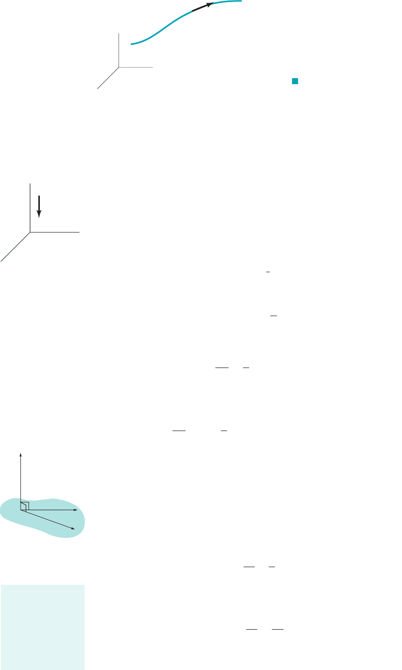
We wish to integrate this differential equation along some arbitrary streamline 1Fig. 6.122and select

the coordinate system with the z axis vertical 1with “up” being positive2so that, as shown by the

figure in the margin, the acceleration of gravity vector can be expressed as

where g is the magnitude of the acceleration of gravity vector. Also, it will be convenient to use

the vector identity

Equation 6.53 can now be written in the form

and this equation can be rearranged to yield

We next take the dot product of each term with a differential length ds along a streamline 1Fig.

6.122. Thus,

(6.54)

Since ds has a direction along the streamline, the vectors ds and V are parallel. However, as shown

by the figure in the margin, the vector is perpendicular to V 1why?2, so it follows that

Recall also that the dot product of the gradient of a scalar and a differential length gives the

differential change in the scalar in the direction of the differential length. That is, with

we can write Thus, Eq.

6.54 becomes

(6.55)

where the change in p, V, and z is along the streamline. Equation 6.55 can now be integrated to

give

(6.56)

which indicates that the sum of the three terms on the left side of the equation must remain a

constant along a given streamline. Equation 6.56 is valid for both compressible and incompressible

冮



 gz  constant



d1V

2 g dz  0

⵱p ⴢ ds  10p



0x2 dx  10p



0y2dy  10p



0z2dz  dp.dx i

 dy j

 dz k

ds 

3V ⴛ 1⵱ⴛV24ⴢ ds  0

V ⴛ 1⵱ⴛV2

⵱p

ⴢ ds 

⵱1V

2ⴢ ds  g⵱z ⴢ ds  3V ⴛ 1⵱ⴛV24ⴢ ds

⵱p



⵱1V

2 g⵱z  V ⴛ 1⵱ⴛV2

rg⵱z  ⵱p 

⵱1V ⴢ V2 rV ⴛ 1⵱ⴛV2

1V ⴢ⵱2V 

⵱1V ⴢ V2 V ⴛ 1⵱ⴛV2

g g⵱z

rg  ⵱p  r1V ⴢ⵱2V

280 Chapter 6 ■ Differential Analysis of Fluid Flow

 gz

 0i  0j  gk

^^^

Streamline

F I G U R E 6.12 The notation for

differential length along a streamline.

V (  V)

 V

Euler’s equations

can be arranged to

give the relation-

ship among pres-

sure, velocity, and

elevation for invis-

cid fluids

JWCL068_ch06_263-331.qxd 9/23/08 12:17 PM Page 280

inviscid flows, but for compressible fluids the variation in with p must be specified before the

first term in Eq. 6.56 can be evaluated.

For inviscid, incompressible fluids 1commonly called ideal fluids2Eq. 6.56 can be written as

(6.57)

and this equation is the Bernoulli equation used extensively in Chapter 3. It is often convenient to

write Eq. 6.57 between two points 112and 122along a streamline and to express the equation in the

“head” form by dividing each term by g so that

(6.58)

It should be again emphasized that the Bernoulli equation, as expressed by Eqs. 6.57 and 6.58, is

restricted to the following:

inviscid flow incompressible flow

steady flow flow along a streamline

You may want to go back and review some of the examples in Chapter 3 that illustrate the use of

the Bernoulli equation.

6.4.3 Irrotational Flow

If we make one additional assumption—that the flow is irrotational—the analysis of inviscid

flow problems is further simplified. Recall from Section 6.1.3 that the rotation of a fluid

element is equal to and an irrotational flow field is one for which 1i.e.,

the curl of velocity is zero2. Since the vorticity, is defined as it also follows that in

an irrotational flow field the vorticity is zero. The concept of irrotationality may seem to be

a rather strange condition for a flow field. Why would a flow field be irrotational? To answer

this question we note that if then each of the components of this vector, as

are given by Eqs. 6.12, 6.13, and 6.14, must be equal to zero. Since these components include

the various velocity gradients in the flow field, the condition of irrotationality imposes specific

relationships among these velocity gradients. For example, for rotation about the z axis to be

zero, it follows from Eq. 6.12 that

and, therefore,

(6.59)

Similarly from Eqs. 6.13 and 6.14

(6.60)

(6.61)

A general flow field would not satisfy these three equations. However, a uniform flow as is illustrated

in Fig. 6.13 does. Since 1a constant2, and it follows that Eqs. 6.59, 6.60, and

6.61 are all satisfied. Therefore, a uniform flow field 1in which there are no velocity gradients2is

certainly an example of an irrotational flow.

Uniform flows by themselves are not very interesting. However, many interesting and

important flow problems include uniform flow in some part of the flow field. Two examples are

w ⫽ 0,v ⫽ 0,u ⫽ U

⫽

⫺

b⫽ 0

1⵱ⴛV2⫽ 0,

⵱ⴛV,Z,

⵱ⴛV ⫽ 0

1⵱ⴛV2,

⫹

⫹ z

⫽

⫹

⫹ z

⫹

⫹ gz ⫽ constant along a streamline

6.4 Inviscid Flow 281

The vorticity is zero

in an irrotational

flow field.

JWCL068_ch06_263-331.qxd 9/23/08 12:17 PM Page 281

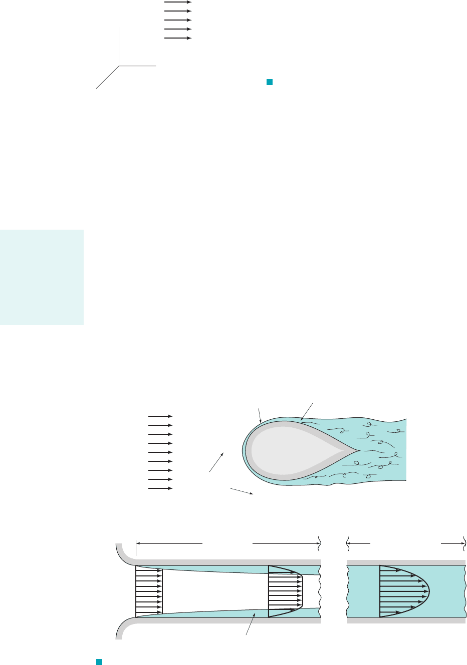
shown in Fig. 6.14. In Fig. 6.14a a solid body is placed in a uniform stream of fluid. Far away

from the body the flow remains uniform, and in this far region the flow is irrotational. In Fig.

6.14b, flow from a large reservoir enters a pipe through a streamlined entrance where the velocity

distribution is essentially uniform. Thus, at the entrance the flow is irrotational.

For an inviscid fluid there are no shearing stresses—the only forces acting on a fluid element

are its weight and pressure forces. Since the weight acts through the element center of gravity, and

the pressure acts in a direction normal to the element surface, neither of these forces can cause the

element to rotate. Therefore, for an inviscid fluid, if some part of the flow field is irrotational, the

fluid elements emanating from this region will not take on any rotation as they progress through

the flow field. This phenomenon is illustrated in Fig. 6.14a in which fluid elements flowing far

away from the body have irrotational motion, and as they flow around the body the motion remains

irrotational except very near the boundary. Near the boundary the velocity changes rapidly from

zero at the boundary 1no-slip condition2to some relatively large value in a short distance from the

boundary. This rapid change in velocity gives rise to a large velocity gradient normal to the boundary

and produces significant shearing stresses, even though the viscosity is small. Of course if we had

a truly inviscid fluid, the fluid would simply “slide” past the boundary and the flow would be

irrotational everywhere. But this is not the case for real fluids, so we will typically have a layer

1usually very thin2near any fixed surface in a moving stream in which shearing stresses are not

negligible. This layer is called the boundary layer. Outside the boundary layer the flow can be

treated as an irrotational flow. Another possible consequence of the boundary layer is that the main

stream may “separate” from the surface and form a wake downstream from the body. (See the

282 Chapter 6 ■ Differential Analysis of Fluid Flow

u = U (constant)

v = 0

w = 0

F I G U R E 6.13 Uniform flow in the x

direction.

Wake

Separation

Boundary

layer

Inviscid

irrotational

flow region

Uniform

approach velocity

(a)

(

Inviscid,

irrotational core

Uniform

entrance

velocity

Boundary layer

Entrance region Fully developed region

F I G U R E 6.14 Various regions of flow: (a) around bodies; (b) through channels.

Flow fields involv-

ing real fluids often

include both

regions of negligi-

ble shearing

stresses and regions

of significant shear-

ing stresses.

JWCL068_ch06_263-331.qxd 9/23/08 12:17 PM Page 282

photographs at the beginning of Chapters 7, 9, and 11.) The wake would include a region of slow,

perhaps randomly moving fluid. To completely analyze this type of problem it is necessary to

consider both the inviscid, irrotational flow outside the boundary layer, and the viscous, rotational

flow within the boundary layer and to somehow “match” these two regions. This type of analysis

is considered in Chapter 9.

As is illustrated in Fig. 6.14b, the flow in the entrance to a pipe may be uniform 1if the

entrance is streamlined2, and thus will be irrotational. In the central core of the pipe the flow

remains irrotational for some distance. However, a boundary layer will develop along the wall

and grow in thickness until it fills the pipe. Thus, for this type of internal flow there will be an

entrance region in which there is a central irrotational core, followed by a so-called fully

developed region in which viscous forces are dominant. The concept of irrotationality is

completely invalid in the fully developed region. This type of internal flow problem is considered

in detail in Chapter 8.

The two preceding examples are intended to illustrate the possible applicability of

irrotational flow to some “real fluid” flow problems and to indicate some limitations of the

irrotationality concept. We proceed to develop some useful equations based on the assumptions

of inviscid, incompressible, irrotational flow, with the admonition to use caution when applying

the equations.

6.4.4 The Bernoulli Equation for Irrotational Flow

In the development of the Bernoulli equation in Section 6.4.2, Eq. 6.54 was integrated along a

streamline. This restriction was imposed so the right side of the equation could be set equal to

zero; that is,

1since ds is parallel to V2. However, for irrotational flow, so the right side of Eq. 6.54

is zero regardless of the direction of ds. We can now follow the same procedure used to obtain Eq.

6.55, where the differential changes and dz can be taken in any direction. Integration of

Eq. 6.55 again yields

(6.62)

where for irrotational flow the constant is the same throughout the flow field. Thus, for

incompressible, irrotational flow the Bernoulli equation can be written as

(6.63)

between any two points in the flow field. Equation 6.63 is exactly the same form as Eq. 6.58 but

is not limited to application along a streamline. However, Eq. 6.63 is restricted to

inviscid flow incompressible flow

steady flow irrotational flow

It may be worthwhile to review the use and misuse of the Bernoulli equation for rotational flow

as is illustrated in Example 3.18.

6.4.5 The Velocity Potential

For an irrotational flow the velocity gradients are related through Eqs. 6.59, 6.60, and 6.61. It

follows that in this case the velocity components can be expressed in terms of a scalar function

(6.64)u ⫽

v ⫽

w ⫽

f1x, y, z, t2

⫹

⫹ z

⫽

⫹

⫹ z

冮

⫹

⫹ gz ⫽ constant

dp, d1V

⵱ⴛV ⫽ 0,

3V ⴛ 1⵱ⴛV24ⴢ ds ⫽ 0

6.4 Inviscid Flow 283

The Bernoulli

equation can be ap-

plied between any

two points in an ir-

rotational flow field.

JWCL068_ch06_263-331.qxd 9/23/08 12:17 PM Page 283

where is called the velocity potential. Direct substitution of these expressions for the velocity

components into Eqs. 6.59, 6.60, and 6.61 will verify that a velocity field defined by Eqs. 6.64 is

indeed irrotational. In vector form, Eqs. 6.64 can be written as

(6.65)

so that for an irrotational flow the velocity is expressible as the gradient of a scalar function

The velocity potential is a consequence of the irrotationality of the flow field, whereas the

stream function is a consequence of conservation of mass (see Section 6.2.3). It is to be noted,

however, that the velocity potential can be defined for a general three-dimensional flow, whereas

the stream function is restricted to two-dimensional flows.

For an incompressible fluid we know from conservation of mass that

and therefore for incompressible, irrotational flow it follows that

(6.66)

where is the Laplacian operator. In Cartesian coordinates

This differential equation arises in many different areas of engineering and physics and is called

Laplace’s equation. Thus, inviscid, incompressible, irrotational flow fields are governed by

Laplace’s equation. This type of flow is commonly called a potential flow. To complete the

mathematical formulation of a given problem, boundary conditions have to be specified. These are

usually velocities specified on the boundaries of the flow field of interest. It follows that if

the potential function can be determined, then the velocity at all points in the flow field can be

determined from Eq. 6.64, and the pressure at all points can be determined from the Bernoulli

equation 1Eq. 6.632. Although the concept of the velocity potential is applicable to both steady and

unsteady flow, we will confine our attention to steady flow.

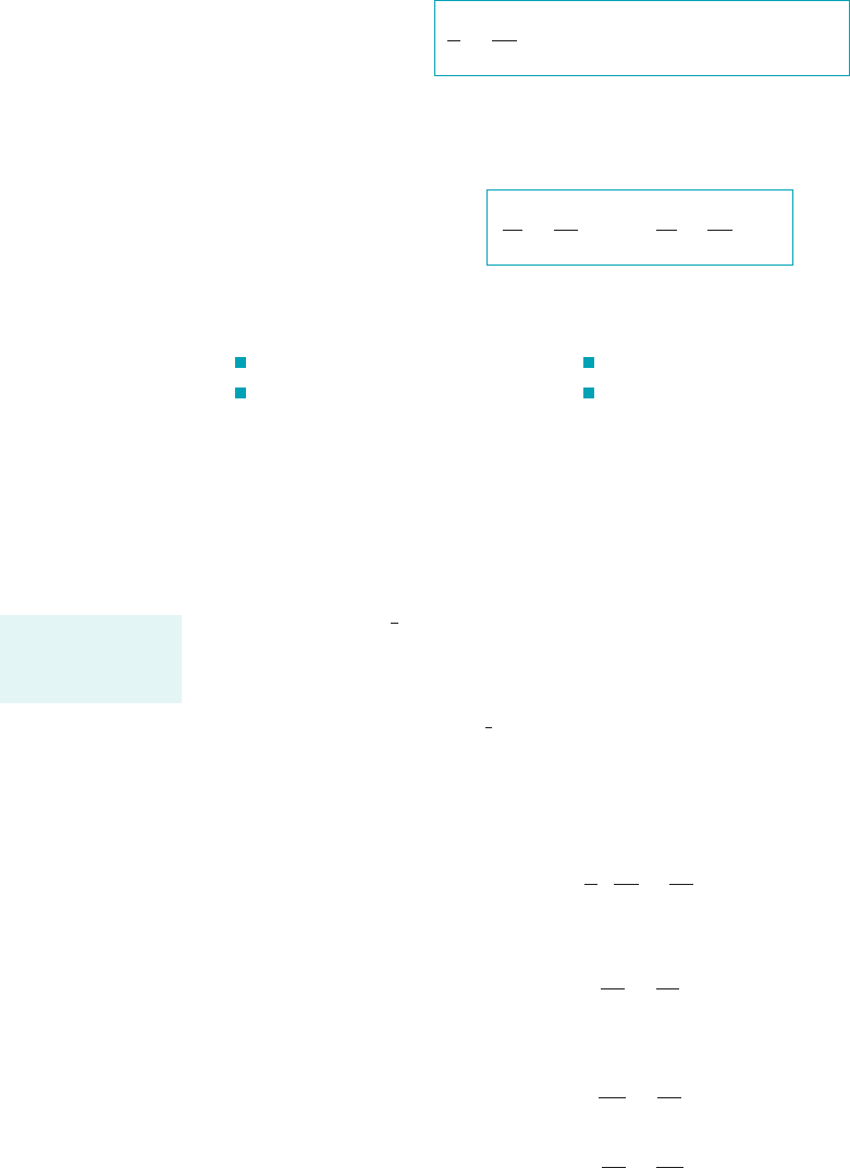
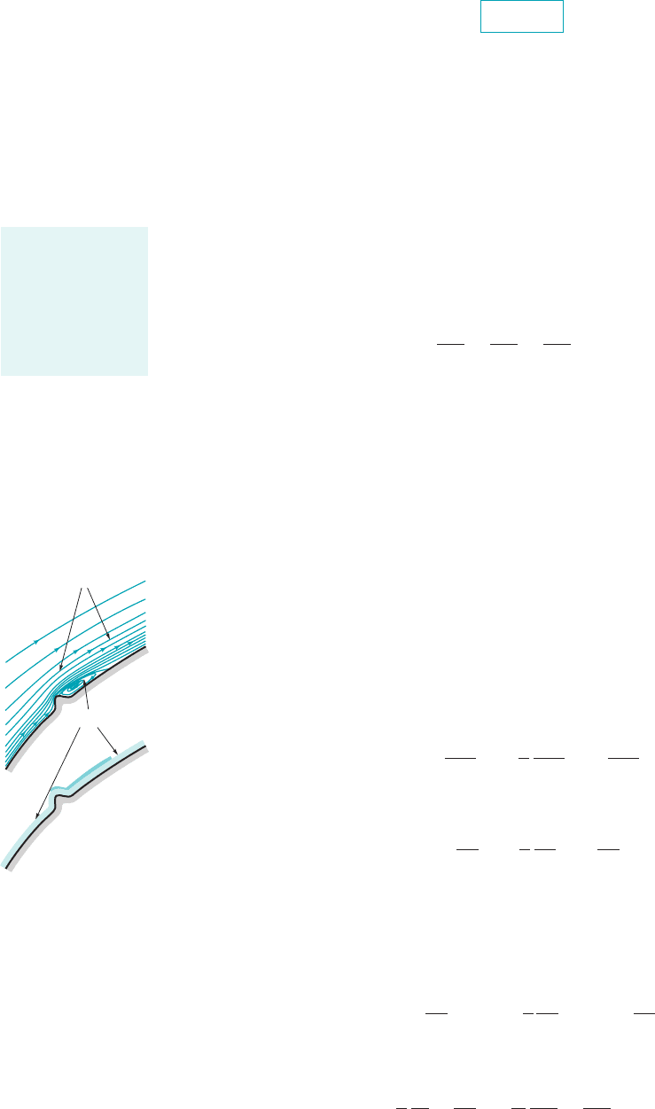
Potential flows, governed by Eqs. 6.64 and 6.66, are irrotational flows. That is, the vorticity

is zero throughout. If vorticity is present (e.g., boundary layer, wake), then the flow cannot be

described by Laplace’s equation. The figure in the margin illustrates a flow in which the vorticity

is not zero in two regions—the separated region behind the bump and the boundary layer next to

the solid surface. This is discussed in detail in Chapter 9.

For some problems it will be convenient to use cylindrical coordinates, r, and z. In this

coordinate system the gradient operator is

(6.67)

so that

(6.68)

where Since

(6.69)

it follows for an irrotational flow

(6.70)

Also, Laplace’s equation in cylindrical coordinates is

(6.71)

b



 0



1with V  ⵱f2

V  v

 v

f  f1r, u, z2.

⵱f 



⵱12

012



012



012



 0

⵱

12 ⵱ⴢ⵱

⵱

f  0

1with V  ⵱f2

⵱ⴢV  0

V  ⵱f

284 Chapter 6 ■ Differential Analysis of Fluid Flow

Inviscid, incom-

pressible, irrota-

tional flow fields

are governed by

Laplace’s equation

and are called

potential flows.

Streamlines

Vorticity contours



  0



  0

JWCL068_ch06_263-331.qxd 9/23/08 12:17 PM Page 284

6.4 Inviscid Flow 285

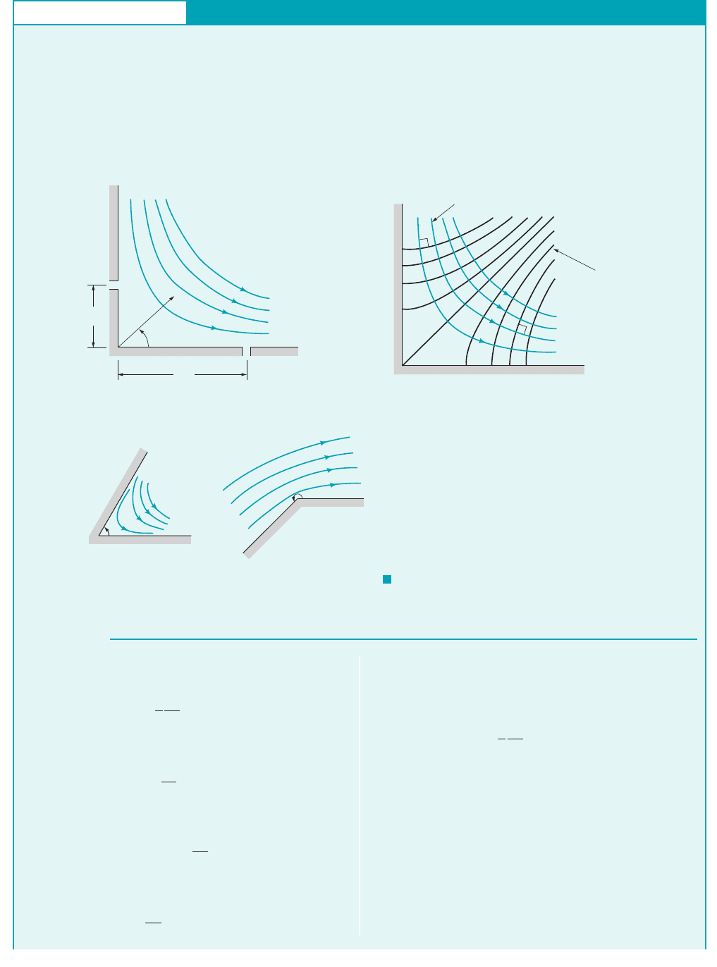
GIVEN The two-dimensional flow of a nonviscous, incom-

pressible fluid in the vicinity of the corner of Fig. E6.4a is

described by the stream function

where has units of when r is in meters. Assume the

fluid density is and the x–y plane is horizontal—

Ⲑ

c ⫽ 2r

sin 2u

90°

that is, there is no difference in elevation between points 112

and 122.

FIND

(a) Determine, if possible, the corresponding velocity potential.

(b) If the pressure at point 112on the wall is 30 kPa, what is the

pressure at point 122?

OLUTION

Velocity Potential and Inviscid Flow Pressure

and therefore by integration

(1)

where is an arbitrary function of Similarly

and integration yields

(2)

where is an arbitrary function of r. To satisfy both Eqs. 1 and

2, the velocity potential must have the form

(Ans)

where C is an arbitrary constant. As is the case for stream functions,

the specific value of C is not important, and it is customary to let

so that the velocity potential for this corner flow is

(Ans)

f ⫽ 2r

cos 2u

C ⫽ 0

f ⫽ 2r

cos 2u ⫹ C

1r2

f ⫽ 2r

cos 2u ⫹ f

1r2

⫽

⫽⫺4r sin 2u

1u2

f ⫽ 2r

cos 2u ⫹ f

1u2

XAMPLE 6.4

(a) The radial and tangential velocity components can be ob-

tained from the stream function as 1see Eq. 6.422

and

Since

it follows that

⫽ 4r cos 2u

⫽

⫽⫺

⫽⫺4r sin 2u

⫽

⫽ 4r cos 2u

(2)

0.5 m

(1)

1 m

Streamline ( = constant)

Equipotential

line

( = constant)

(a)(b)

(c)

F I G U R E E6.4

JWCL068_ch06_263-331.qxd 9/23/08 12:17 PM Page 285

286 Chapter 6 ■ Differential Analysis of Fluid Flow

COMMENT In the statement of this problem it was implied

by the wording “if possible” that we might not be able to find a

corresponding velocity potential. The reason for this concern is

that we can always define a stream function for two-dimensional

flow, but the flow must be irrotational if there is a corresponding

velocity potential. Thus, the fact that we were able to determine a

velocity potential means that the flow is irrotational. Several

streamlines and lines of constant are plotted in Fig. E6.4b.

These two sets of lines are orthogonal. The reason why stream-

lines and lines of constant are always orthogonal is explained in

Section 6.5.

(b) Since we have an irrotational flow of a nonviscous, incom-

pressible fluid, the Bernoulli equation can be applied between any

two points. Thus, between points 112and 122with no elevation

change

(3)

Since

it follows that for any point within the flow field

 16r

1cos

2u  sin

2u2

 14r cos 2u2

 14r sin 2u2

 v

 v

 p



 V







This result indicates that the square of the velocity at any point

depends only on the radial distance, r, to the point. Note that the

constant, 16, has units of Thus,

and

Substitution of these velocities into Eq. 3 gives

(Ans)

COMMENT The stream function used in this example could

also be expressed in Cartesian coordinates as

since and However, in the cylindrical po-

lar form the results can be generalized to describe flow in the vicin-

ity of a corner of angle 1see Fig. E6.4c2with the equations

and

where A is a constant.

f  Ar



cos

c  Ar



sin

y  r sin u.x  r cos u

c  4xy

c  2r

sin 2u  4r

sin u cos u

 36 kPa

 30  10







116 m



 4 m



 116 s

2

210.5 m2

 4 m



 116 s

2

211 m2

 16 m



2

A major advantage of Laplace’s equation is that it is a linear partial differential equation. Since it

is linear, various solutions can be added to obtain other solutions—that is, if and

are two solutions to Laplace’s equation, then is also a solution. The

practical implication of this result is that if we have certain basic solutions we can combine them

to obtain more complicated and interesting solutions. In this section several basic velocity potentials,

which describe some relatively simple flows, will be determined. In the next section these basic

potentials will be combined to represent complicated flows.

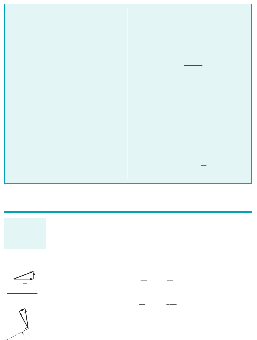
For simplicity, only plane 1two-dimensional2flows will be considered. In this case, by using

Cartesian coordinates

(6.72)

or by using cylindrical coordinates

(6.73)

as shown by the figure in the margin. Since we can define a stream function for plane flow, we

can also let

(6.74)u 

v 



u 

v 

 f

 f

1x, y, z2

6.5 Some Basic, Plane Potential Flows

For potential flow,

basic solutions can

be simply added to

obtain more com-

plicated solutions.

u =

∂

v =

∂

∂r

JWCL068_ch06_263-331.qxd 9/23/08 12:17 PM Page 286