Munson B.R. Fundamentals of Fluid Mechanics

Подождите немного. Документ загружается.

8.5.2 Multiple Pipe Systems

In many pipe systems there is more than one pipe involved. The complex system of tubes in

our lungs 1beginning as shown by the figure in the margin, with the relatively large-diameter

trachea and ending in tens of thousands of minute bronchioles after numerous branchings2and

the maze of pipes in a city’s water distribution system are typical of such systems. The gov-

erning mechanisms for the flow in multiple pipe systems are the same as for the single pipe

systems discussed in this chapter. However, because of the numerous unknowns involved,

additional complexities may arise in solving for the flow in multiple pipe systems. Some of

these complexities are discussed in this section.

8.5 Pipe Flow Examples 437

Bronchiole

Lung

Trachea

Fluids in the News

Deepwater pipeline Pipelines used to transport oil and gas are

commonplace. But south of New Orleans, in deep waters of the

Gulf of Mexico, a not-so-common multiple pipe system is being

built. The new so-called Mardi Gras system of pipes is being laid

in water depths of 4300 to 7300 feet. It will transport oil and gas

from five deepwater fields with the interesting names of Holstein,

Mad Dog, Thunder Horse, Atlantis, and Na Kika. The deepwater

pipelines will connect with lines at intermediate water depths to

transport the oil and gas to shallow-water fixed platforms and

shore. The steel pipe used is 28 inches in diameter with a wall

thickness of 1 1兾8 in. The thick-walled pipe is needed to with-

stand the large external pressure which is about 3250 psi at a

depth of 7300 ft. The pipe is installed in 240-ft sections from a

vessel the size of a large football stadium. Upon completion, the

deepwater pipeline system will have a total length of more than

450 miles and the capability of transporting more than 1 million

barrels of oil per day and 1.5 billion cubic feet of gas per day.

(See Problem 8.113.)

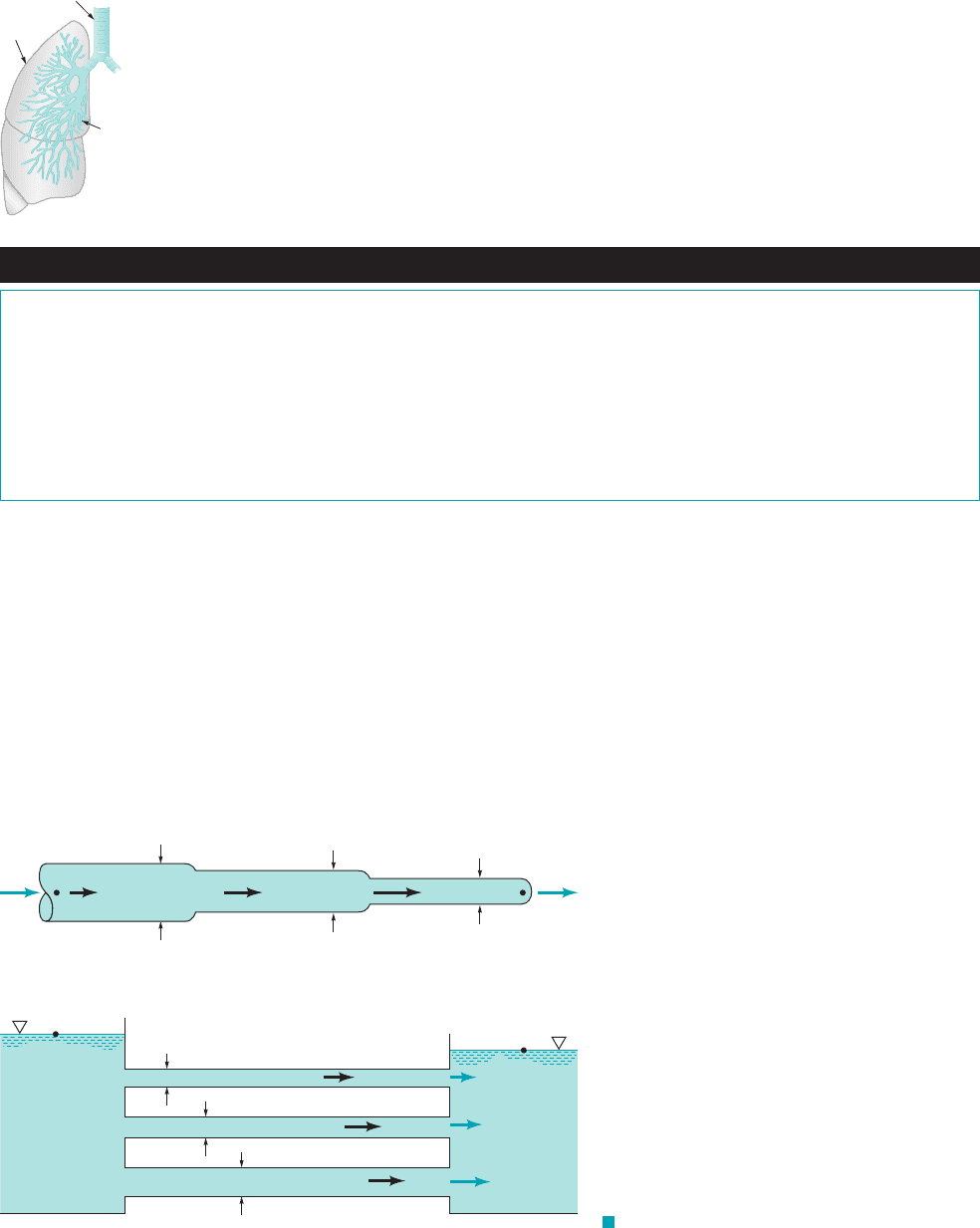
The simplest multiple pipe systems can be classified into series or parallel flows, as are shown

in Fig. 8.35. The nomenclature is similar to that used in electrical circuits. Indeed, an analogy be-

tween fluid and electrical circuits is often made as follows. In a simple electrical circuit, there is

a balance between the voltage 1e2, current 1i2, and resistance 1R2as given by Ohm’s law: In a

fluid circuit there is a balance between the pressure drop the flowrate or velocity 1Q or V2,

and the flow resistance as given in terms of the friction factor and minor loss coefficients .

For a simple flow it follows that where a measure of the

resistance to the flow, is proportional to f.

The main differences between the solution methods used to solve electrical circuit problems

and those for fluid circuit problems lie in the fact that Ohm’s law is a linear equation 1doubling

the voltage doubles the current2, while the fluid equations are generally nonlinear 1doubling the

pressure drop does not double the flowrate unless the flow is laminar2. Thus, although some of the

,¢p ⫽ Q

,3¢p ⫽ f 1/

Ⲑ

D21rV

Ⲑ

224,

1 f and K

1¢p2,

e ⫽ iR.

(1) (2) (3)

(a)

(1)

(2)

(3)

(b)

F I G U R E 8.35 (a) Series and (b)

parallel pipe systems.

JWCL068_ch08_383-460.qxd 9/23/08 10:59 AM Page 437

standard electrical engineering methods can be carried over to help solve fluid mechanics prob-

lems, others cannot.

One of the simplest multiple pipe systems is that containing pipes in series, as is shown in

Fig. 8.35a. Every fluid particle that passes through the system passes through each of the pipes.

Thus, the flowrate 1but not the velocity2is the same in each pipe, and the head loss from point A

to point B is the sum of the head losses in each of the pipes. The governing equations can be writ-

ten as follows:

and

where the subscripts refer to each of the pipes. In general, the friction factors will be different for

each pipe because the Reynolds numbers and the relative roughnesses will

be different. If the flowrate is given, it is a straightforward calculation to determine the head loss or

pressure drop 1Type I problem2. If the pressure drop is given and the flowrate is to be calculated

1Type II problem2, an iteration scheme is needed. In this situation none of the friction factors, are

known, so the calculations may involve more trial-and-error attempts than for corresponding single

pipe systems. The same is true for problems in which the pipe diameter 1or diameters2is to be de-

termined 1Type III problems2.

Another common multiple pipe system contains pipes in parallel, as is shown in Fig. 8.35b.

In this system a fluid particle traveling from A to B may take any of the paths available, with the

total flowrate equal to the sum of the flowrates in each pipe. However, by writing the energy equa-

tion between points A and B it is found that the head loss experienced by any fluid particle traveling

between these locations is the same, independent of the path taken. Thus, the governing equations

for parallel pipes are

and

Again, the method of solution of these equations depends on what information is given and what

is to be calculated.

Another type of multiple pipe system called a loop is shown in Fig. 8.36. In this case the

flowrate through pipe 112equals the sum of the flowrates through pipes 122and 132, or

As can be seen by writing the energy equation between the surfaces of each reservoir, the head

loss for pipe 122must equal that for pipe 132, even though the pipe sizes and flowrates may be dif-

ferent for each. That is,

for a fluid particle traveling through pipes 112and 122, while

⫹

⫹ z

⫽

⫹

⫹ z

⫹ h

⫹

⫹ z

⫽

⫹

⫹ z

⫹ h

⫽ Q

⫹ Q

⫽ h

Q ⫽ Q

⫹ Q

Ⲑ

21Re

⫽ rV

Ⲑ

A – B

⫽ h

⫹ h

⫽ Q

438 Chapter 8 ■ Viscous Flow in Pipes

F I G U R E 8.36 Multiple pipe loop system.

(2)

(3)

(1)

Node,

Series and parallel

pipe systems are of-

ten encountered.

JWCL068_ch08_383-460.qxd 9/23/08 10:59 AM Page 438

for fluid that travels through pipes 112and 132. These can be combined to give This is a

statement of the fact that fluid particles that travel through pipe 122and particles that travel through

pipe 132all originate from common conditions at the junction 1or node, N2of the pipes and all end

up at the same final conditions.

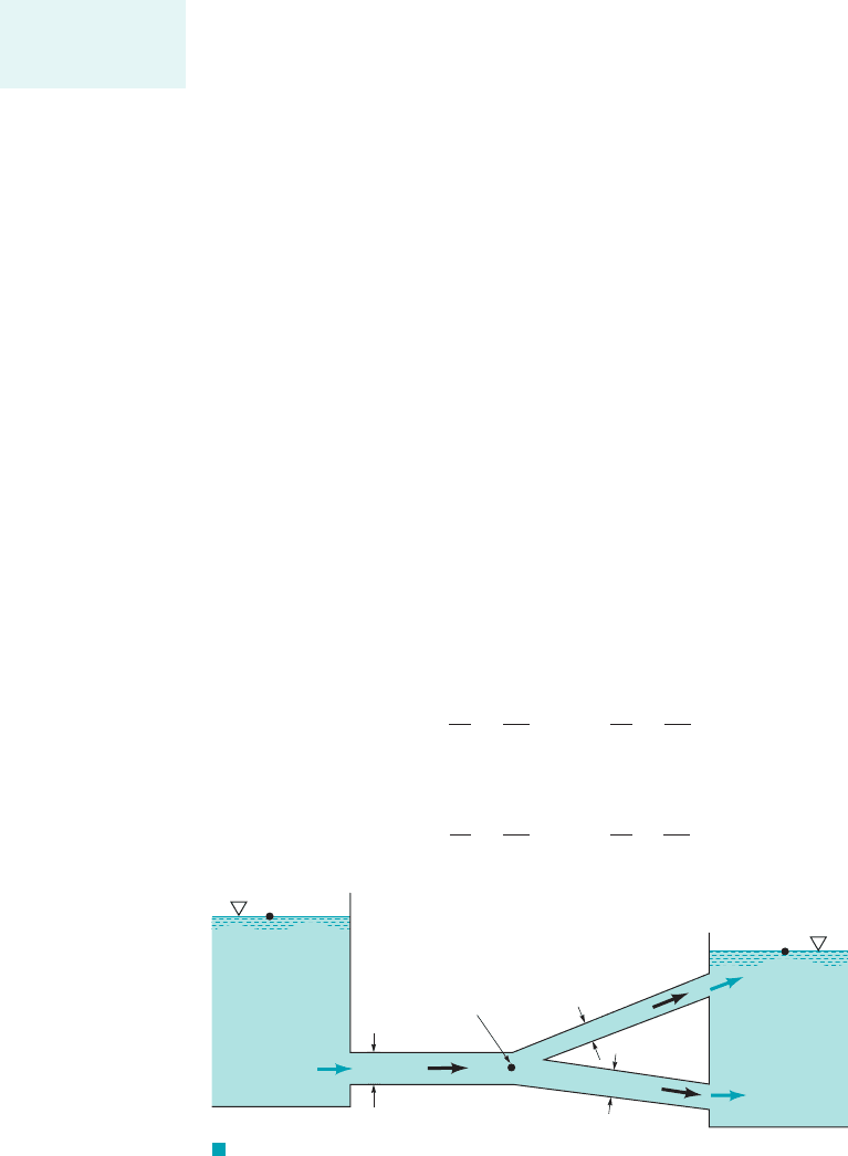
The flow in a relatively simple looking multiple pipe system may be more complex than

it appears initially. The branching system termed the three-reservoir problem shown in Fig. 8.37

is such a system. Three reservoirs at known elevations are connected together with three pipes

of known properties 1lengths, diameters, and roughnesses2. The problem is to determine the

flowrates into or out of the reservoirs. If valve 112were closed, the fluid would flow from

reservoir B to C, and the flowrate could be easily calculated. Similar calculations could be

carried out if valves 122or 132were closed with the others open.

With all valves open, however, it is not necessarily obvious which direction the fluid flows.

For the conditions indicated in Fig. 8.37, it is clear that fluid flows from reservoir A because the

other two reservoir levels are lower. Whether the fluid flows into or out of reservoir B depends

on the elevation of reservoirs B and C and the properties 1length, diameter, roughness2of the

three pipes. In general, the flow direction is not obvious, and the solution process must include

the determination of this direction. This is illustrated in Example 8.14.

⫽ h

8.5 Pipe Flow Examples 439

F I G U R E 8.37

A three-reservoir system.

(3)

(2)

(1)

, ᐉ

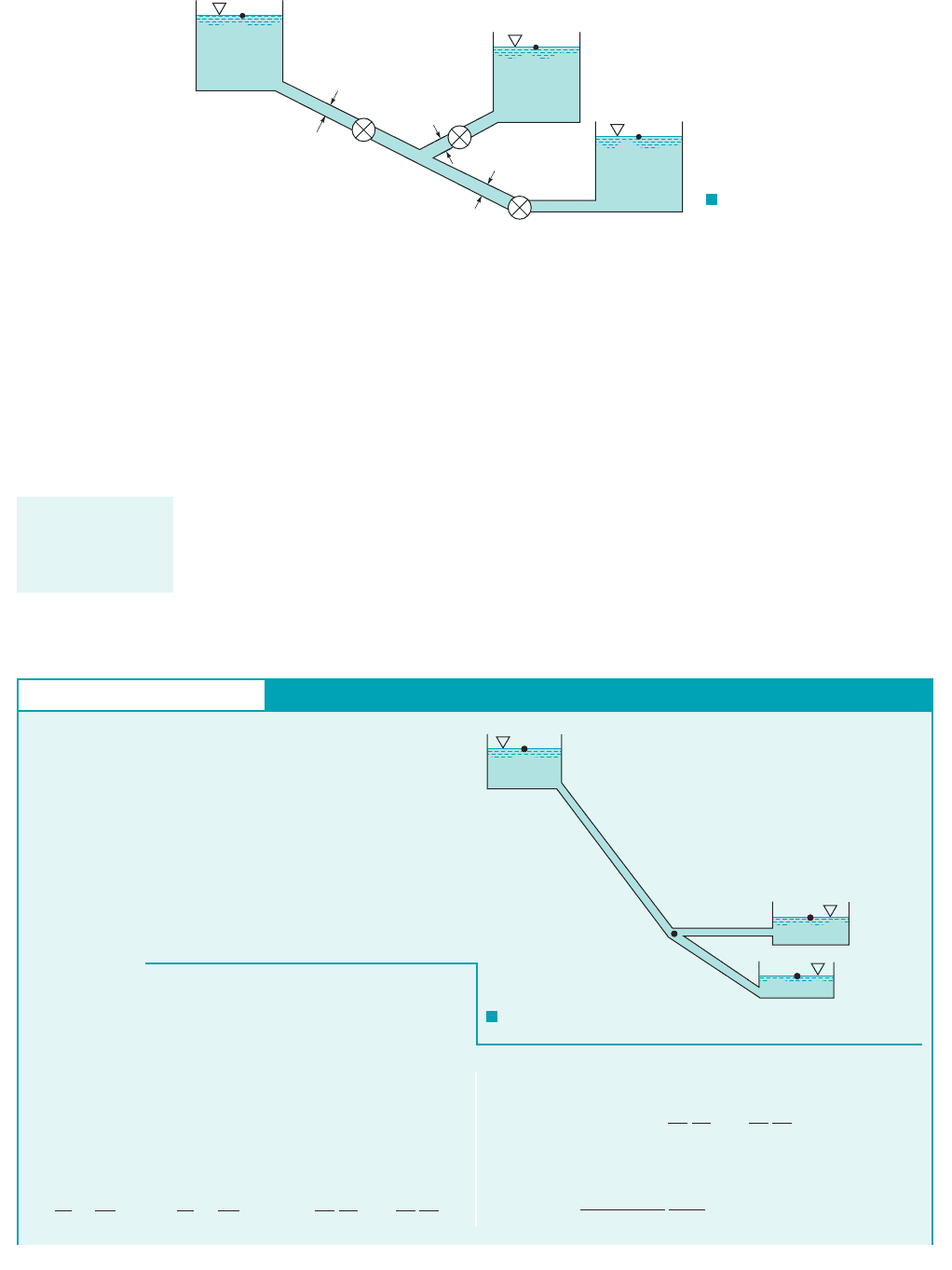
GIVEN Three reservoirs are connected by three pipes as are

shown in Fig. E8.14. For simplicity we assume that the diame-

ter of each pipe is 1 ft, the friction factor for each is 0.02, and

because of the large length-to-diameter ratio, minor losses are

negligible.

FIND Determine the flowrate into or out of each reservoir.

Three-Reservoir, Multiple-Pipe System

XAMPLE 8.14

OLUTION

By using the fact that this becomes

For the given conditions of this problem we obtain

100 ft ⫽

0.02

2132.2 ft

Ⲑ

11 ft2

311000 ft2V

⫹ 1400 ft2V

⫽ f

⫹ f

⫽ p

⫽ V

⫽ z

⫽ 0,

It is not obvious which direction the fluid flows in pipe 122.

However, we assume that it flows out of reservoir B, write the

governing equations for this case, and check our assumption.

The continuity equation requires that which,

since the diameters are the same for each pipe, becomes simply

(1)

The energy equation for the fluid that flows from A to C in pipes

112and 132can be written as

⫹

⫹ z

⫽

⫹

⫹ z

⫹ f

⫹ V

⫽ V

⫹ Q

⫽ Q

F I G U R E E8.14

Elevation = 100 ft

Elevation =

20 ft

Elevation =

0 ft

(1)

(2)

(3)

= 1 ft

ᐉ

= 1000 ft

= 1 ft

ᐉ

= 500 ft

= 1 ft

ᐉ

= 400 ft

For some pipe sys-

tems, the direction

of flow is not

known a priori.

JWCL068_ch08_383-460.qxd 9/23/08 10:59 AM Page 439

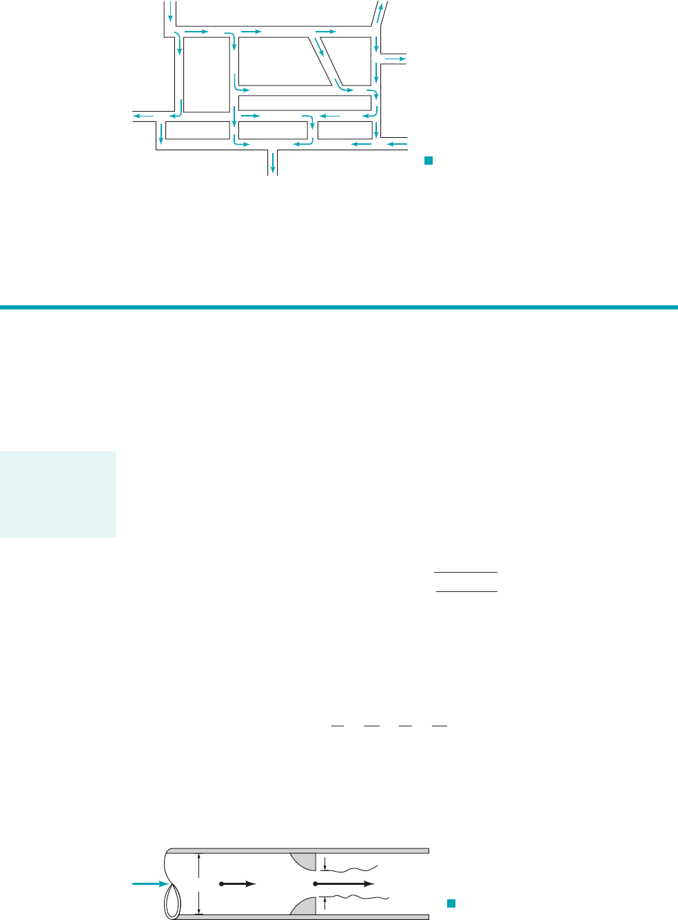
The ultimate in multiple pipe systems is a network of pipes such as that shown in Fig. 8.38.

Networks like these often occur in city water distribution systems and other systems that may have

multiple “inlets” and “outlets.” The direction of flow in the various pipes is by no means obvi-

ous—in fact, it may vary in time, depending on how the system is used from time to time.

The solution for pipe network problems is often carried out by use of node and loop equations

similar in many ways to that done in electrical circuits. For example, the continuity equation requires

that for each node 1the junction of two or more pipes2the net flowrate is zero. What flows into a node

must flow out at the same rate. In addition, the net pressure difference completely around a loop

1starting at one location in a pipe and returning to that location2must be zero. By combining these

ideas with the usual head loss and pipe flow equations, the flow throughout the entire network can

440 Chapter 8 ■ Viscous Flow in Pipes

(2)

where and are in ft兾s. Similarly the energy equation for

fluid flowing from B and C is

For the given conditions this can be written as

(3)

Equations 1, 2, and 3 1in terms of the three unknowns and

2are the governing equations for this flow, provided the fluid flows

from reservoir B. It turns out, however, that there is no solution for

these equations with positive, real values of the velocities. Although

these equations do not appear to be complicated, there is no simple

way to solve them directly. Thus, a trial-and-error solution is sug-

gested. This can be accomplished as follows. Assume a value of

calculate from Eq. 2, and then from Eq. 3. It is found

that the resulting trio does not satisfy Eq. 1 for any value of

assumed. There is no solution to Eqs. 1, 2, and 3 with real, positive

values of and Thus, our original assumption of flow out of

reservoir B must be incorrect.

To obtain the solution, assume the fluid flows into reser-

voirs B and C and out of A. For this case the continuity equation

becomes

(4)

Application of the energy equation between points A and B and A

and C gives

and

⫽ z

⫹ f

⫽ z

⫹ f

⫽ V

⫹ V

⫽ Q

⫹ Q

, V

7 0,

, V

64.4 ⫽ 0.5V

⫹ 0.4V

⫽ f

⫹ f

⫹

⫹ z

⫽

⫹

⫹ z

⫹ f

322 ⫽ V

⫹ 0.4V

which, with the given data, become

(5)

and

(6)

Equations 4, 5, and 6 can be solved as follows. By subtracting

Eq. 5 from 6 we obtain

Thus, Eq. 5 can be written as

(7)

which, upon squaring both sides, can be written as

By using the quadratic formula we can solve for to obtain

either Thus, either

The value is not a root of the orig-

inal equations. It is an extra root introduced by squaring Eq. 7, which

with becomes Thus,

and from Eq. 5, The corresponding flowrates are

(Ans)

and

(Ans)

Note the slight differences in the governing equations depending

on the direction of the flow in pipe 122—compare Eqs. 1, 2, and 3

with Eqs. 4, 5, and 6.

COMMENT If the friction factors were not given, a trial-and-

error procedure similar to that needed for Type II problems 1see

Section 8.5.12would be required.

⫽ 10.2 ft

Ⲑ

s into C

⫽ Q

⫺ Q

⫽ 112.5 ⫺ 2.262 ft

Ⲑ

⫽ 2.26 ft

Ⲑ

s into B

⫽ A

⫽

11 ft2

12.88 ft

Ⲑ

⫽ 12.5 ft

Ⲑ

s from A

⫽ A

⫽

11 ft2

115.9 ft

Ⲑ

⫽ 15.9 ft

Ⲑ

⫽ 2.88 ft

Ⲑ

s“1140 ⫽⫺1140.”V

⫽ 21.3

⫽ 21.3 ft

Ⲑ

⫽ 2.88 ft

Ⲑ

⫽ 21.3 ft

Ⲑ

s orV

⫽ 452 or V

⫽ 8.30.

⫺ 460 V

⫹ 3748 ⫽ 0

2160 ⫹ 1.25V

⫽ 98 ⫺ 2.75V

⫽ 1V

⫹ 2160 ⫹ 1.25V

⫹ 0.5V

258 ⫽ 1V

⫹ V

⫹ 0.5V

⫽ 2160 ⫹ 1.25V

322 ⫽ V

⫹ 0.4 V

258 ⫽ V

⫹ 0.5 V

Pipe network prob-

lems can be solved

using node and

loop concepts.

JWCL068_ch08_383-460.qxd 9/23/08 11:00 AM Page 440

be obtained. Of course, trial-and-error solutions are usually required because the direction of flow

and the friction factors may not be known. Such a solution procedure using matrix techniques is ide-

ally suited for computer use 1Refs. 21, 222.

8.6 Pipe Flowrate Measurement 441

F I G U R E 8.38 A general

pipe network.

8.6 Pipe Flowrate Measurement

It is often necessary to determine experimentally the flowrate in a pipe. In Chapter 3 we introduced

various types of flow-measuring devices 1Venturi meter, nozzle meter, orifice meter, etc.2and dis-

cussed their operation under the assumption that viscous effects were not important. In this section

we will indicate how to account for the ever-present viscous effects in these flow meters. We will

also indicate other types of commonly used flow meters.

8.6.1 Pipe Flowrate Meters

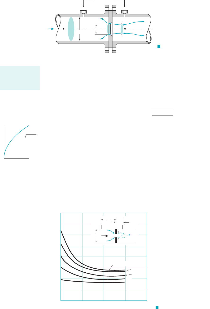
Three of the most common devices used to measure the instantaneous flowrate in pipes are the ori-

fice meter, the nozzle meter, and the Venturi meter. As was discussed in Section 3.6.3, each of these

meters operates on the principle that a decrease in flow area in a pipe causes an increase in veloc-

ity that is accompanied by a decrease in pressure. Correlation of the pressure difference with the

velocity provides a means of measuring the flowrate. In the absence of viscous effects and under

the assumption of a horizontal pipe, application of the Bernoulli equation 1Eq. 3.72between points

112and 122shown in Fig. 8.39 gave

(8.37)

where Based on the results of the previous sections of this chapter, we anticipate that

there is a head loss between 112and 122so that the governing equations become

and

The ideal situation has and results in Eq. 8.37. The difficulty in including the head loss is

that there is no accurate expression for it. The net result is that empirical coefficients are used in

the flowrate equations to account for the complex real-world effects brought on by the nonzero

viscosity. The coefficients are discussed in this section.

⫽ 0

⫹

⫽

⫹

⫹ h

Q ⫽ A

⫽ A

b ⫽ D

Ⲑ

ideal

⫽ A

21p

⫺ p

r11 ⫺ b

F I G U R E 8.39 Typical

pipe flow meter geometry.

(1)

(2)

Orifice, nozzle and

Venturi meters

involve the concept

“high velocity gives

low pressure.”

JWCL068_ch08_383-460.qxd 9/23/08 11:00 AM Page 441

A typical orifice meter is constructed by inserting between two flanges of a pipe a flat plate

with a hole, as shown in Fig. 8.40. The pressure at point 122within the vena contracta is less than

that at point 112. Nonideal effects occur for two reasons. First, the vena contracta area, is less than

the area of the hole, by an unknown amount. Thus, where is the contraction co-

efficient Second, the swirling flow and turbulent motion near the orifice plate introduce a

head loss that cannot be calculated theoretically. Thus, an orifice discharge coefficient, is used to

take these effects into account. That is,

(8.38)

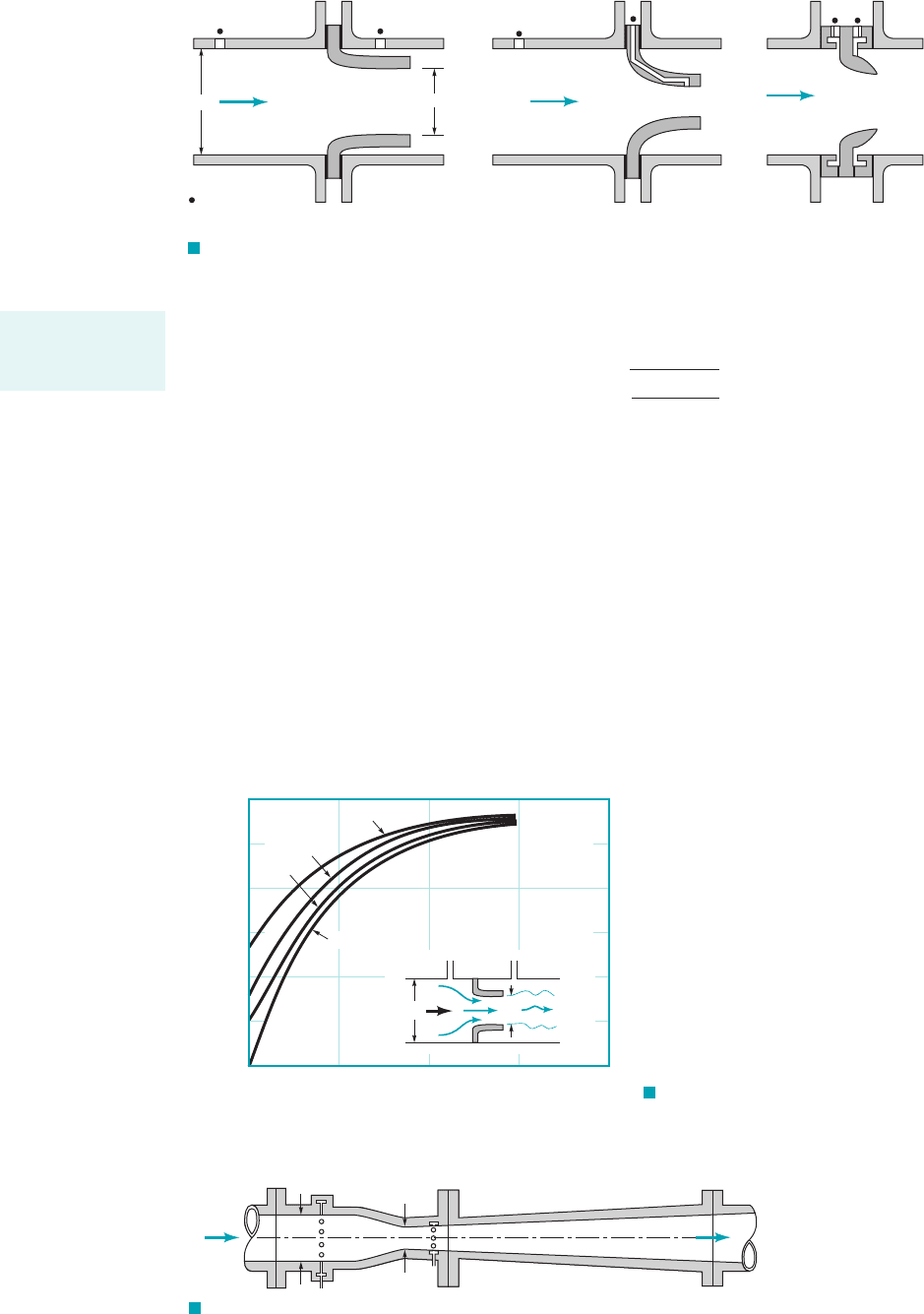
where is the area of the hole in the orifice plate. The value of is a function of

and the Reynolds number where Typical values of are given

in Fig. 8.41. As shown by Eq. 8.38 and the figure in the margin, for a given value of , the

flowrate is proportional to the square root of the pressure difference. Note that the value of

depends on the specific construction of the orifice meter 1i.e., the placement of the pressure taps,

whether the orifice plate edge is square or beveled, etc.2. Very precise conditions governing the

construction of standard orifice meters have been established to provide the greatest accuracy pos-

sible 1Refs. 23, 242.

Another type of pipe flow meter that is based on the same principles used in the orifice me-

ter is the nozzle meter, three variations of which are shown in Fig. 8.42. This device uses a con-

toured nozzle 1typically placed between flanges of pipe sections2rather than a simple 1and less

expensive2plate with a hole as in an orifice meter. The resulting flow pattern for the nozzle meter

is closer to ideal than the orifice meter flow. There is only a slight vena contracta and the secondary

V  Q



.Re  rVD



m,b  d



 pd



Q  C

ideal

 C

21p

 p

r11  b

6 12.

 C

442 Chapter 8 ■ Viscous Flow in Pipes

An orifice discharge

coefficient is used

to account for non-

ideal effects.

(1)

(2)

Pressure taps

= D

F I G U R E 8.40

Typical orifice meter construction.

= = 0.7

0.5

0.6

0.4

0.2

0.66

0.64

0.62

0.60

0.58

Re = VD/

ρμ

F I G U R E 8.41 Orifice

meter discharge coefficient (Ref. 24).

~ p

 p

JWCL068_ch08_383-460.qxd 9/23/08 11:00 AM Page 442

flow separation is less severe, but there still are viscous effects. These are accounted for by use of

the nozzle discharge coefficient, where

(8.39)

with As with the orifice meter, the value of is a function of the diameter ratio,

and the Reynolds number, Typical values obtained from experiments are

shown in Fig. 8.43. Again, precise values of depend on the specific details of the nozzle de-

sign. Accepted standards have been adopted 1Ref. 242. Note that the nozzle meter is more

efficient 1less energy dissipated2than the orifice meter.

The most precise and most expensive of the three obstruction-type flow meters is the Venturi

meter shown in Fig. 8.44 [G. B. Venturi (1746–1822)]. Although the operating principle for this de-

vice is the same as for the orifice or nozzle meters, the geometry of the Venturi meter is designed to

reduce head losses to a minimum. This is accomplished by providing a relatively streamlined con-

traction 1which eliminates separation ahead of the throat2and a very gradual expansion downstream

of the throat 1which eliminates separation in this decelerating portion of the device2. Most of the head

loss that occurs in a well-designed Venturi meter is due to friction losses along the walls rather than

losses associated with separated flows and the inefficient mixing motion that accompanies such flow.

7 C

;

Re ⫽ rVD

Ⲑ

m.b ⫽ d

Ⲑ

⫽ pd

Ⲑ

Q ⫽ C

ideal

⫽ C

21p

⫺ p

r11 ⫺ b

8.6 Pipe Flowrate Measurement 443

F I G U R E 8.42 Typical nozzle meter construction.

The nozzle meter is

more efficient than

the orifice meter.

(a)(b)(c)

Pressure taps

F I G U R E 8.43 Nozzle

meter discharge coefficient (Ref. 24).

1.00

0.98

0.96

0.94

Re = VD/

ρμ

0.6

0.4

0.2

= = 0.8

F I G U R E 8.44 Typical Venturi meter construction.

JWCL068_ch08_383-460.qxd 9/23/08 11:00 AM Page 443

Thus, the flowrate through a Venturi meter is given by

(8.40)

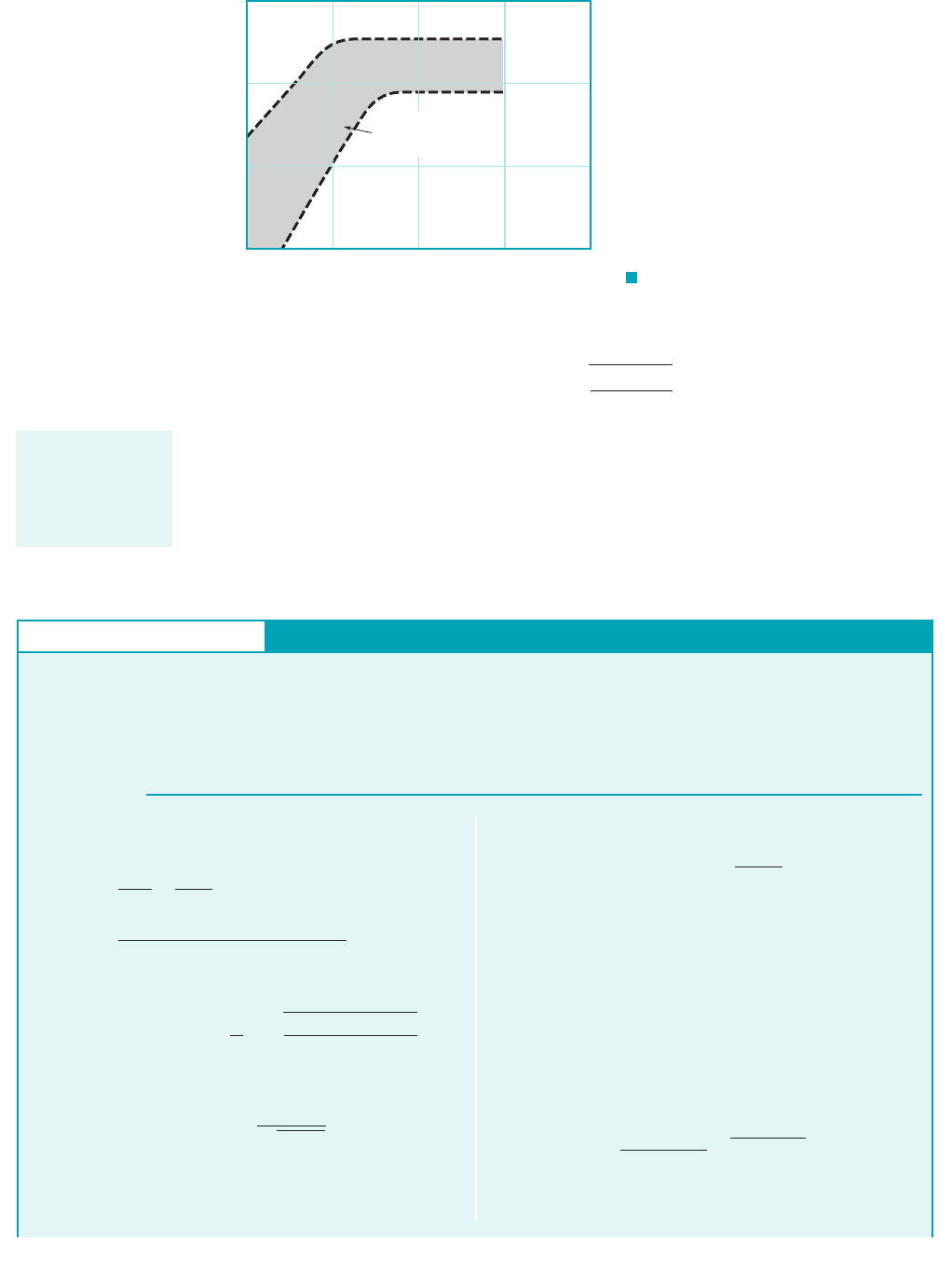
where is the throat area. The range of values of , the Venturi discharge coefficient,

is given in Fig. 8.45. The throat-to-pipe diameter ratio the Reynolds number, and the

shape of the converging and diverging sections of the meter are among the parameters that affect

the value of

Again, the precise values of and depend on the specific geometry of the devices

used. Considerable information concerning the design, use, and installation of standard flow meters

can be found in various books 1Refs. 23, 24, 25, 26, 312.

, C

1b  d



D2,

 pd



Q  C

ideal

 CA

21p

 p

r11  b

444 Chapter 8 ■ Viscous Flow in Pipes

The Venturi dis-

charge coefficient

is a function of the

specific geometry

of the meter.

F I G U R E 8.45 Venturi

meter discharge coefficient (Ref. 23).

1.00

0.98

0.96

0.94

Re = VD/

ρμ

Range of values

depending on specific

geometry

GIVEN Ethyl alcohol flows through a pipe of diameter

in a refinery. The pressure drop across the nozzle

meter used to measure the flowrate is to be when

the flowrate is

Q  0.003 m



¢p  4.0 kPa

D  60 mm

Nozzle Flow Meter

XAMPLE 8.15

OLUTION

As a first approximation we assume that the flow is ideal, or

so that Eq. 1 becomes

(2)

In addition, for many cases so that an approximate

value of d can be obtained from Eq. 2 as

Hence, with an initial guess of or

we obtain from Fig. 8.43 1using

2a value of Clearly this does not agree with

our initial assumption of Thus, we do not have the so-

lution to Eq. 1 and Fig. 8.43. Next we assume and

and solve for d from Eq. 1 to obtain

or With the new value of

and we obtain 1from Fig. 8.432 in

⬇ 0.972

Re  42,200,

0.568

b  0.0341



0.060 d  0.0341 m.

d  a

1.20  10

3

0.972

21  0.577



 0.972

b  0.577

 1.0.

 0.972.

42,200

Re 

0.0346



0.06  0.577,

b  d



D d  0.0346 m

d  11.20  10

3



 0.0346 m

1  b

⬇ 1,

d  11.20  10

3

21  b



 1.0,

From Table 1.6 the properties of ethyl alcohol are

and Thus,

From Eq. 8.39 the flowrate through the nozzle is

(1)

where d is in meters. Note that Equation 1

and Fig. 8.43 represent two equations for the two unknowns d and

that must be solved by trial and error.

b  d



D  d



0.06.

1.20  10

3



21  b

Q  0.003 m



s  C

214  10



789 kg



11  b



41789 kg



210.003 m



p10.06 m211.19  10

3



 42,200

Re 

rVD



4rQ

pDm

3



m  1.19 

r 789 kg



FIND Determine the diameter, d, of the nozzle.

JWCL068_ch08_383-460.qxd 9/23/08 11:00 AM Page 444

Numerous other devices are used to measure the flowrate in pipes. Many of these devices

use principles other than the high-speed/low-pressure concept of the orifice, nozzle, and Venturi

meters.

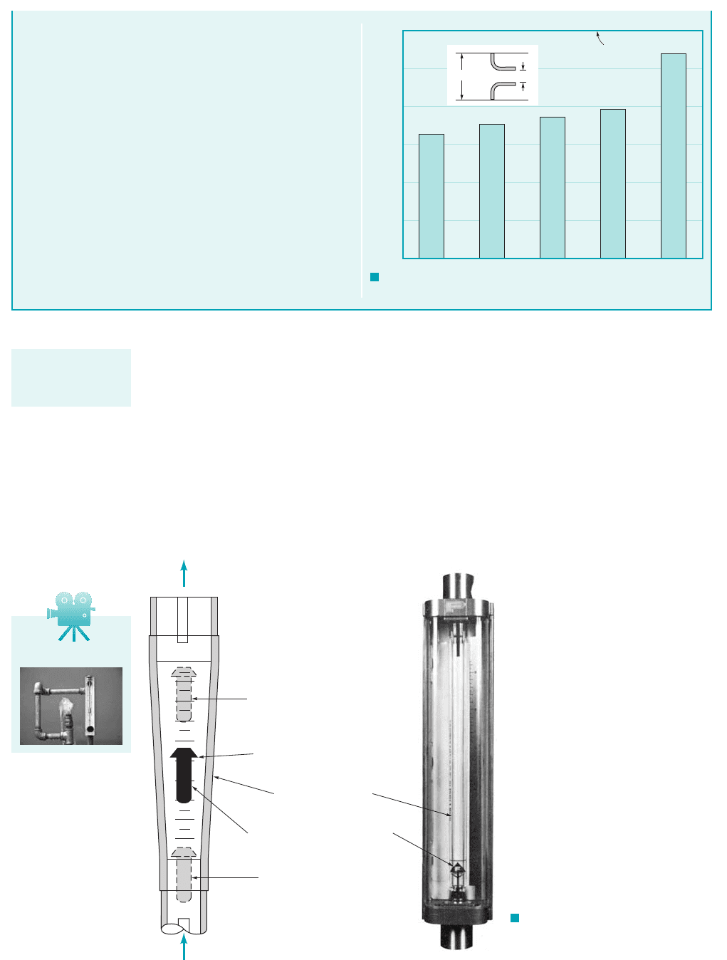
A quite common, accurate, and relatively inexpensive flow meter is the rotameter, or vari-

able area meter as is shown in Fig. 8.46. In this device a float is contained within a tapered, trans-

parent metering tube that is attached vertically to the pipeline. As fluid flows through the meter

1entering at the bottom2, the float will rise within the tapered tube and reach an equilibrium height

that is a function of the flowrate. This height corresponds to an equilibrium condition for which

the net force on the float 1buoyancy, float weight, fluid drag2is zero. A calibration scale in the tube

provides the relationship between the float position and the flowrate.

8.6 Pipe Flowrate Measurement 445

agreement with the assumed value. Thus,

(Ans)

COMMENTS If numerous cases are to be investigated, it may

be much easier to replace the discharge coefficient data of Fig.

8.43 by the equivalent equation, and use a com-

puter to iterate for the answer. Such equations are available in the

literature 1Ref. 242. This would be similar to using the Colebrook

equation rather than the Moody chart for pipe friction problems.

By repeating the calculations, the nozzle diameters, d, needed

for the same flowrate and pressure drop but with different fluids

are shown in Fig. E8.15. The diameter is a function of the fluid

viscosity because the nozzle coefficient, C

, is a function of the

Reynolds number (see Fig. 8.43). In addition, the diameter is a

function of the density because of this Reynolds number effect

and, perhaps more importantly, because the density is involved di-

rectly in the flowrate equation, Eq. 8.39. These factors all com-

bine to produce the results shown in the figure.

⫽ f1b, Re2,

d ⫽ 34.1 mm

F I G U R E E8.15

d, mm

Gasoline

Alcohol

Water

Carbon tet

Mercury

d = D

There are many

types of flow

meters.

Float at large end of tube indicates

maximum flowrate

Position of edge of float against

scale gives flowrate reading

Tapered metering tube

Metering float is freely suspended

in process fluid

Float at narrow end of tube

indicates minimum flowrate

F I G U R E 8.46

Rotameter-type flow meter.

(Courtesy of Fischer &

Porter Co.)

V8.13 Rotameter

JWCL068_ch08_383-460.qxd 9/23/08 11:00 AM Page 445

Another useful pipe flowrate meter is a turbine meter as is shown in Fig. 8.47. A small, freely

rotating propeller or turbine within the turbine meter rotates with an angular velocity that is a func-

tion of 1nearly proportional to2the average fluid velocity in the pipe. This angular velocity is picked

up magnetically and calibrated to provide a very accurate measure of the flowrate through the meter.

8.6.2 Volume Flow Meters

In many instances it is necessary to know the amount 1volume or mass2of fluid that has passed

through a pipe during a given time period, rather than the instantaneous flowrate. For example,

we are interested in how many gallons of gasoline are pumped into the tank in our car rather than

the rate at which it flows into the tank. There are numerous quantity-measuring devices that pro-

vide such information.

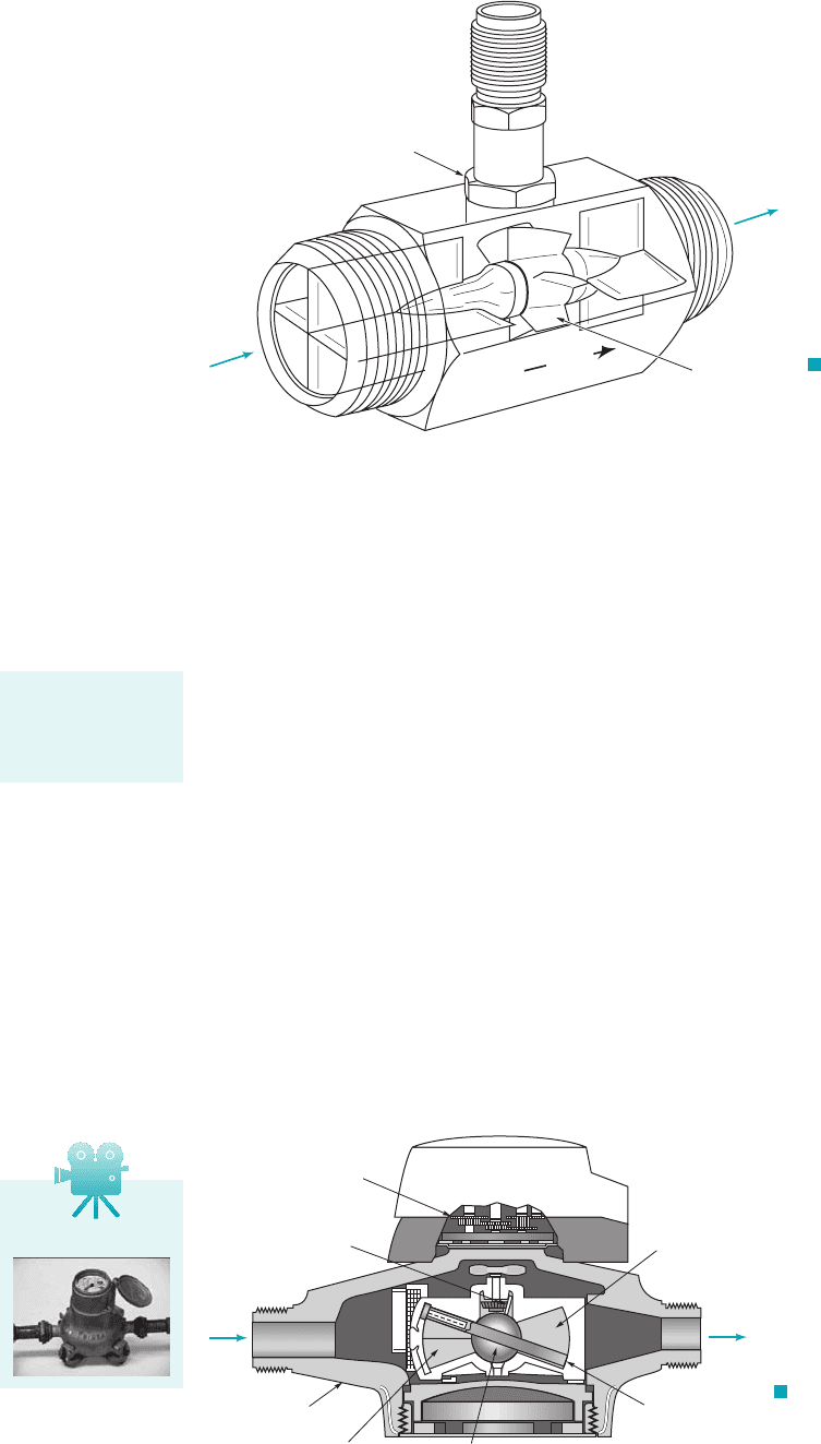
The nutating disk meter shown in Fig. 8.48 is widely used to measure the net amount of wa-

ter used in domestic and commercial water systems as well as the amount of gasoline delivered to

your gas tank. This meter contains only one essential moving part and is relatively inexpensive and

accurate. Its operating principle is very simple, but it may be difficult to understand its operation

without actually inspecting the device firsthand. The device consists of a metering chamber with

spherical sides and conical top and bottom. A disk passes through a central sphere and divides the

chamber into two portions. The disk is constrained to be at an angle not normal to the axis of sym-

metry of the chamber. A radial plate 1diaphragm2divides the chamber so that the entering fluid

causes the disk to wobble 1nutate2, with fluid flowing alternately above or below the disk. The fluid

exits the chamber after the disk has completed one wobble, which corresponds to a specific volume

of fluid passing through the chamber. During each wobble of the disk, the pin attached to the tip

446 Chapter 8 ■ Viscous Flow in Pipes

F I G U R E 8.47

Turbine-type flow meter.

(Courtesy of E G & G Flow

Technology, Inc.)

FLOW

OUT

Magnetic sensor

Turbine

Flow

out

Volume flow meters

measure volume

rather than volume

flowrate.

F I G U R E 8.48

Nutating disk flow meter.

(Courtesy of Badger Meter,

Inc.)

Calibration gears

Flow

out

Metering

chamber

Disk assembly

SphereDiaphragm

Casing

V8.14 Water meter

JWCL068_ch08_383-460.qxd 9/23/08 11:00 AM Page 446