Munson B.R. Fundamentals of Fluid Mechanics

Подождите немного. Документ загружается.

A wide variety of lift and drag information for airfoils can be found in standard aerodynam-

ics books 1Ref. 13, 14, 292.

9.4 Lift 517

F I G U R E 9.35 Typi-

cal lift and drag alterations possible

with the use of various types of flap

designs (Ref. 21).

No flaps

Trailing edge

slotted flap

Double slotted

trailing edge flaps

(Data not

shown)

Leading

edge flap

3.0

2.0

1.0

0 0.1 0.2 0.3

V9.18 Leading

edge flap

Fluids in the News

Learning from nature For hundreds of years humans looked

toward nature, particularly birds, for insight about flying. How-

ever, all early airplanes that closely mimicked birds proved to be

unsuccessful. Only after much experimenting with rigid (or at

least nonflapping) wings did human flight become possible. Re-

cently, however, engineers have been turning to living sys-

tems—birds, insects, and other biological models—in an at-

tempt to produce breakthroughs in aircraft design. Perhaps it is

possible that nature’s basic design concepts can be applied to

airplane systems. For example, by morphing and rotating their

wings in three dimensions, birds have remarkable maneuver-

ability that to date has no technological parallel. Birds can con-

trol the airflow over their wings by moving the feathers on their

wingtips and the leading edges of their wings, providing designs

that are more efficient than the flaps and rigid, pivoting tail sur-

faces of current aircraft (Ref. 15). On a smaller scale, under-

standing the mechanism by which insects dynamically manage

unstable flow to generate lift may provide insight into the devel-

opment of microscale air vehicles. With new hi-tech materials,

computers, and automatic controls, aircraft of the future may

mimic nature more than was once thought possible. (See Prob-

lem 9.110.)

GIVEN In 1977 the Gossamer Condor, shown in Fig. E9.15a,

won the Kremer prize by being the first human-powered aircraft to

complete a prescribed figure-of-eight course around two turning

points 0.5 mi apart 1Ref. 222.The following data pertain to this aircraft:

⫽ power to overcome drag

Ⲑ

pilot power ⫽0.8

power train efficiency ⫽ h

drag coefficient ⫽ C

⫽ 0.046 1based on planform area2

weight 1including pilot2⫽ w ⫽ 210 lb

wing size ⫽ b ⫽ 96 ft, c ⫽ 7.5 ft 1average2

flight speed ⫽ U ⫽ 15 ft

Ⲑ

Lift and Power for Human Powered Flight

XAMPLE 9.15

FIND Determine

(a) the lift coefficient, C

, and

(b) the power, required by the pilot.p,

F I G U R E E9.15

JWCL068_ch09_461-533.qxd 9/23/08 11:49 AM Page 517

9.4.2 Circulation

Since viscous effects are of minor importance in the generation of lift, it should be possible to cal-

culate the lift force on an airfoil by integrating the pressure distribution obtained from the equa-

tions governing inviscid flow past the airfoil. That is, the potential flow theory discussed in Chap-

ter 6 should provide a method to determine the lift. Although the details are beyond the scope of

this book, the following is found from such calculations 1Ref. 42.

The calculation of the inviscid flow past a two-dimensional airfoil gives a flow field as in-

dicated in Fig. 9.36. The predicted flow field past an airfoil with no lift 1i.e., a symmetrical airfoil

at zero angle of attack, Fig. 9.36a2appears to be quite accurate 1except for the absence of thin

boundary layer regions2. However, as is indicated in Fig. 9.36b, the calculated flow past the same

airfoil at a nonzero angle of attack 1but one small enough so that boundary layer separation would

not occur2is not proper near the trailing edge. In addition, the calculated lift for a nonzero angle

of attack is zero—in conflict with the known fact that such airfoils produce lift.

In reality, the flow should pass smoothly over the top surface as is indicated in Fig. 9.36c, with-

out the strange behavior indicated near the trailing edge in Fig. 9.36b. As is shown in Fig. 9.36d, the

unrealistic flow situation can be corrected by adding an appropriate clockwise swirling flow around

the airfoil. The results are twofold: 112The unrealistic behavior near the trailing edge is eliminated 1i.e.,

518 Chapter 9 ■ Flow over Immersed Bodies

OLUTION

COMMENT

This power level is obtainable by a well-condi-

tioned athlete 1as is indicated by the fact that the flight was suc-

cessfully completed2. Note that only 80% of the pilot’s power

1i.e., which corresponds to a drag of

2is needed to force the aircraft through the air. The

other 20% is lost because of the power train inefficiency.

By repeating the calculations for various flight speeds, the

results shown in Fig. E9.15b are obtained. Note from Eq. 1 that

for a constant drag coefficient, the power required increases as

—a doubling of the speed to 30 ft/s would require an eight-

fold increase in power (i.e., 2.42 hp, well beyond the range of

any human).

d ⫽ 8.86 lb

0.8 ⫻ 0.302 ⫽ 0.242 hp,

(a) For steady flight conditions the lift must be exactly balanced

by the weight, or

Thus,

where and

for standard air. This gives

(Ans)

a reasonable number. The overall lift-to-drag ratio for the aircraft is

23.7.

(b) The product of the power that the pilot supplies and the power

train efficiency equals the useful power needed to overcome the

drag, That is,

where

Thus,

(1)

(Ans)

p ⫽ 166 ft

Ⲑ

s a

1 hp

550 ft

Ⲑ

b⫽ 0.302 hp

p ⫽

12.38 ⫻ 10

⫺3

slugs

Ⲑ

21720 ft

210.0462115 ft

Ⲑ

210.82

p ⫽

⫽

rAC

d ⫽

hp ⫽ dU

Ⲑ

⫽ 1.09

Ⲑ

0.046 ⫽

⫽ 1.09

⫽

21210 lb2

12.38 ⫻ 10

⫺3

slugs

Ⲑ

2115 ft

Ⲑ

1720 ft

2.38 ⫻ 10

⫺3

slugs

Ⲑ

r ⫽A ⫽ bc ⫽ 96 ft ⫻ 7.5 ft ⫽ 720 ft

, w ⫽ 210 lb,

⫽

w ⫽ l ⫽

2.5

2.0

1.5

1.0

0.5

, hp

15 20 25 30

U, ft/s

1005

(15, 0.302)

F I G U R E E9.15

Inviscid flow analy-

sis can be used to

obtain ideal flow

past airfoils.

JWCL068_ch09_461-533.qxd 9/23/08 11:49 AM Page 518

the flow pattern of Fig. 9.36b is changed to that of Fig. 9.36c2, and 122the average velocity on the

upper surface of the airfoil is increased while that on the lower surface is decreased. From the Bernoulli

equation concepts 1i.e., 2, the average pressure on the upper surface is

decreased and that on the lower surface is increased. The net effect is to change the original zero lift

condition to that of a lift-producing airfoil.

The addition of the clockwise swirl is termed the addition of circulation. The amount of

swirl 1circulation2needed to have the flow leave the trailing edge smoothly is a function of the

airfoil size and shape and can be calculated from potential flow 1inviscid2theory 1see Section 6.6.3

and Ref. 292. Although the addition of circulation to make the flow field physically realistic may

seem artificial, it has well-founded mathematical and physical grounds. For example, consider the

flow past a finite length airfoil, as is indicated in Fig. 9.37. For lift-generating conditions the av-

erage pressure on the lower surface is greater than that on the upper surface. Near the tips of the

wing this pressure difference will cause some of the fluid to attempt to migrate from the lower

to the upper surface, as is indicated in Fig. 9.37b. At the same time, this fluid is swept down-

stream, forming a trailing vortex 1swirl2from each wing tip 1see Fig. 4.32. It is speculated that the

reason some birds migrate in vee-formation is to take advantage of the updraft produced by the

trailing vortex of the preceding bird. [It is calculated that for a given expenditure of energy, a flock

of 25 birds flying in vee-formation could travel 70% farther than if each bird were to fly sepa-

rately 1Ref. 152.]

The trailing vortices from the right and left wing tips are connected by the bound vortex

along the length of the wing. It is this vortex that generates the circulation that produces the

lift. The combined vortex system 1the bound vortex and the trailing vortices2is termed a horse-

shoe vortex. The strength of the trailing vortices 1which is equal to the strength of the bound

vortex2is proportional to the lift generated. Large aircraft 1for example, a Boeing 7472can gen-

erate very strong trailing vortices that persist for a long time before viscous effects and insta-

bility mechanisms finally cause them to die out. Such vortices are strong enough to flip smaller

aircraft out of control if they follow too closely behind the large aircraft. The figure in the mar-

gin clearly shows a trailing vortex produced during a wake vortex study in which an airplane

flew through a column of smoke.

Ⲑ

g ⫹ V

Ⲑ

2g ⫹ z ⫽ constant

9.4 Lift 519

F I G U R E 9.36 Inviscid

flow past an airfoil: (a) symmetrical flow

past the symmetrical airfoil at a zero

angle of attack; (b) same airfoil at a

nonzero angle of attack—no lift, flow

near trailing edge not realistic; (c) same

conditions as for (b) except circulation

has been added to the flow—nonzero

lift, realistic flow; (d) superposition of

flows to produce the final flow past the

airfoil.

(a)

(b)

(c)

(d)

= 0

ᏸ = 0

> 0

ᏸ = 0

> 0

ᏸ > 0

"(a) + circulation = (c)"

V9.19 Wing tip

vortices

(Photograph courtesy of

NASA.)

JWCL068_ch09_461-533.qxd 9/23/08 11:49 AM Page 519

520 Chapter 9 ■ Flow over Immersed Bodies

F I G U R E 9.37 Flow past a finite length wing: (a) the horseshoe

vortex system produced by the bound vortex and the trailing vortices; (b) the

leakage of air around the wing tips produces the trailing vortices.

Bound vortex

Trailing

vortex

(a)

(

Low pressure

High pressure

Bound vortex

Trailing vortex

Fluids in the News

Why winglets? Winglets, those upward turning ends of airplane

wings, boost the performance by reducing drag. This is accom-

plished by reducing the strength of the wingtip vortices formed by

the difference between the high pressure on the lower surface of

the wing and the low pressure on the upper surface of the wing.

These vortices represent an energy loss and an increase in drag. In

essence, the winglet provides an effective increase in the aspect

ratio of the wing without extending the wingspan. Winglets come

in a variety of styles—the Airbus A320 has a very small upper and

lower winglet; the Boeing 747-400 has a conventional, vertical

upper winglet; and the Boeing Business Jet (a derivative of the

Boeing 737) has an eight-foot winglet with a curving transition

from wing to winglet. Since the airflow around the winglet is

quite complicated, the winglets must be carefully designed and

tested for each aircraft. In the past, winglets were more likely to

be retrofitted to existing wings, but new airplanes are being de-

signed with winglets from the start. Unlike tailfins on cars,

winglets really do work. (See Problem 9.111.)

As is indicated above, the generation of lift is directly related to the production of a swirl or

vortex flow around the object. A nonsymmetric airfoil, by design, generates its own prescribed

amount of swirl and lift. A symmetric object like a circular cylinder or sphere, which normally

provides no lift, can generate swirl and lift if it rotates.

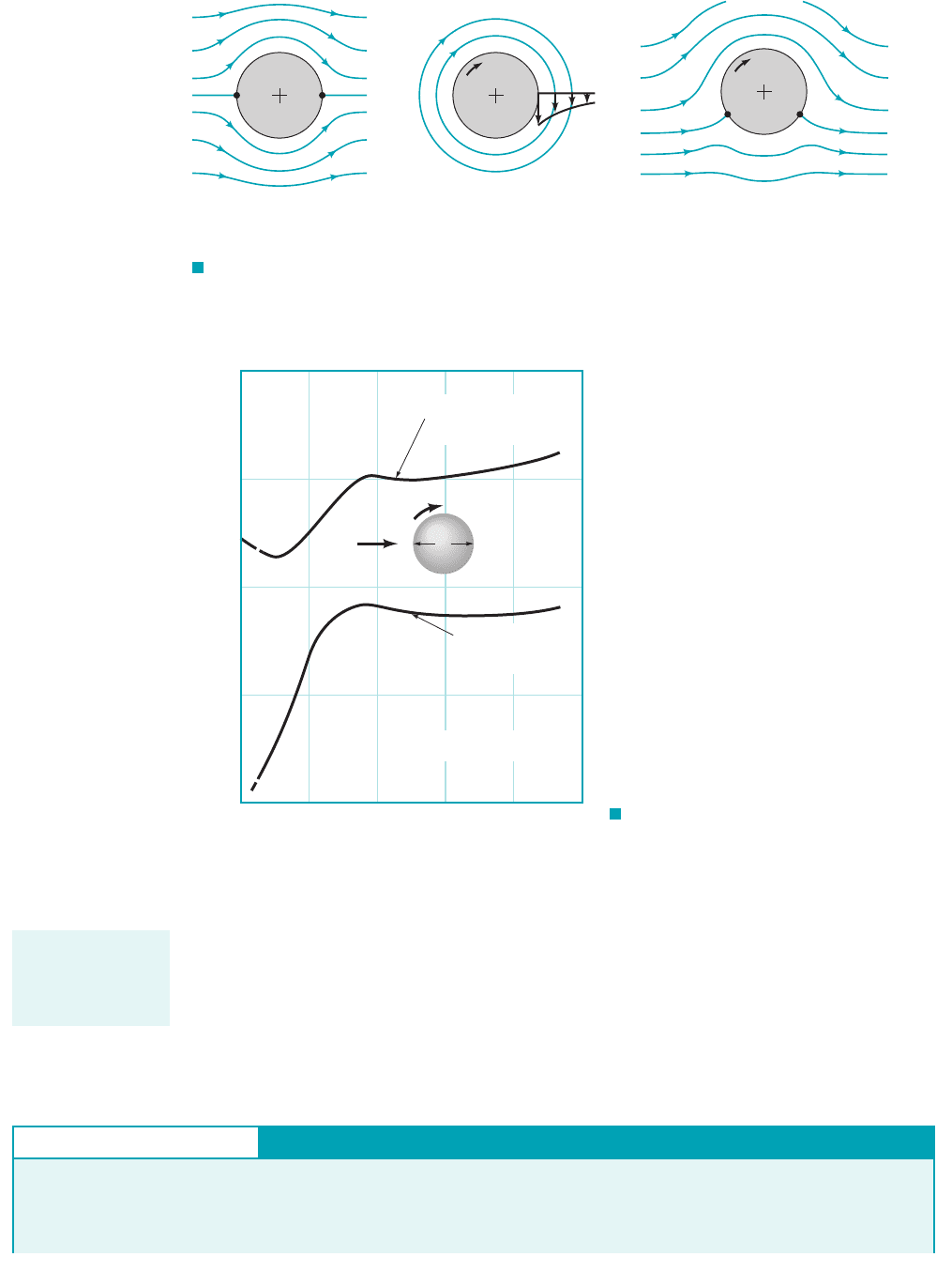
As is discussed in Section 6.6.3, the inviscid flow past a circular cylinder has the symmet-

rical flow pattern indicated in Fig. 9.38a. By symmetry the lift and drag are zero. However, if the

cylinder is rotated about its axis in a stationary real fluid, the rotation will drag some of

the fluid around, producing circulation about the cylinder as in Fig. 9.38b. When this circulation

is combined with an ideal, uniform upstream flow, the flow pattern indicated in Fig. 9.38c is ob-

tained. The flow is no longer symmetrical about the horizontal plane through the center of the

cylinder; the average pressure is greater on the lower half of the cylinder than on the upper half,

and a lift is generated. This effect is called the Magnus effect, after Heinrich Magnus 11802–18702,

a German chemist and physicist who first investigated this phenomenon. A similar lift is generated

on a rotating sphere. It accounts for the various types of pitches in baseball 1i.e., curve ball, floater,

sinker, etc.2, the ability of a soccer player to hook the ball, and the hook or slice of a golf ball.

Typical lift and drag coefficients for a smooth, spinning sphere are shown in Fig. 9.39. Al-

though the drag coefficient is fairly independent of the rate of rotation, the lift coefficient is strongly

1m  02

A spinning sphere

or cylinder can

generate lift.

JWCL068_ch09_461-533.qxd 9/23/08 11:49 AM Page 520

dependent on it. In addition 1although not indicated in the figure2, both and are dependent on

the roughness of the surface. As was discussed in Section 9.3, in a certain Reynolds number range

an increase in surface roughness actually decreases the drag coefficient. Similarly, an increase in sur-

face roughness can increase the lift coefficient because the roughness helps drag more fluid around

the sphere increasing the circulation for a given angular velocity. Thus, a rotating, rough golf ball

travels farther than a smooth one because the drag is less and the lift is greater. However, do not ex-

pect a severely roughed up 1cut2ball to work better—extensive testing has gone into obtaining the

optimum surface roughness for golf balls.

9.4 Lift 521

F I G U R E 9.38 Inviscid flow past a circular cylinder: (a) uniform upstream flow without

circulation, (b) free vortex at the center of the cylinder, (c) combination of free vortex and uniform flow

past a circular cylinder giving nonsymmetric flow and a lift.

= stagnation point (highest pressure)

“(

a) + (b) = (c)”

(

c)(b)(a)

F I G U R E 9.39 Lift and drag

coefficients for a spinning smooth sphere (Ref. 23).

Smooth sphere

0.2

0.4

0.6

0.8

123

D/2U

Re = = 6 × 10

___



____________



____________

, C

GIVEN A table tennis ball weighing with di-

ameter is hit at a velocity of with

a back spin of angular velocity as is shown in Fig. E9.16.v

U ⫽ 12 m

Ⲑ

D ⫽ 3.8 ⫻ 10

⫺2

2.45 ⫻ 10

⫺2

FIND What is the value of if the ball is to travel on a hori-

zontal path, not dropping due to the acceleration of gravity?

Lift on a Rotating Sphere

XAMPLE 9.16

A dimpled golf ball

has less drag and

more lift than a

smooth one.

JWCL068_ch09_461-533.qxd 9/23/08 11:49 AM Page 521

522 Chapter 9 ■ Flow over Immersed Bodies

In this chapter the flow past objects is discussed. It is shown how the pressure and shear

stress distributions on the surface of an object produce the net lift and drag forces on the

object.

The character of flow past an object is a function of the Reynolds number. For large

Reynolds number flows a thin boundary layer forms on the surface. Properties of this boundary

layer flow are discussed. These include the boundary layer thickness, whether the flow is lami-

nar or turbulent, and the wall shear stress exerted on the object. In addition, boundary layer sep-

aration and its relationship to the pressure gradient are considered.

The drag, which contains portions due to friction (viscous) effects and pressure effects, is

written in terms of the dimensionless drag coefficient. It is shown how the drag coefficient is a

function of shape, with objects ranging from very blunt to very streamlined. Other parameters

affecting the drag coefficient include the Reynolds number, Froude number, Mach number, and

surface roughness.

The lift is written in terms of the dimensionless lift coefficient, which is strongly depen-

dent on the shape of the object. Variation of the lift coefficient with shape is illustrated by the

variation of an airfoil’s lift coefficient with angle of attack.

The following checklist provides a study guide for this chapter. When your study of the

entire chapter and end-of-chapter exercises has been completed you should be able to

write out meanings of the terms listed here in the margin and understand each of the related

concepts. These terms are particularly important and are set in italic, bold, and color type

in the text.

9.5 Chapter Summary and Study Guide

drag

lift

lift coefficient

drag coefficient

wake region

boundary layer

laminar boundary layer

turbulent boundary layer

boundary layer thickness

transition

free-stream velocity

favorable pressure

gradient

adverse pressure

gradient

boundary layer

separation

friction drag

pressure drag

stall

circulation

Magnus effect

OLUTION

COMMENT

Is it possible to impart this angular velocity to

the ball? With larger angular velocities the ball will rise and fol-

low an upward curved path. Similar trajectories can be produced

by a well-hit golf ball—rather than falling like a rock, the golf

ball trajectory is actually curved up and the spinning ball travels a

greater distance than one without spin. However, if topspin is im-

parted to the ball 1as in an improper tee shot2the ball will curve

downward more quickly than under the action of gravity alone—

the ball is “topped” and a negative lift is generated. Similarly, ro-

tation about a vertical axis will cause the ball to hook or slice to

one side or the other.

For horizontal flight, the lift generated by the spinning of the

ball must exactly balance the weight, of the ball so that

where the lift coefficient, can be obtained from Fig. 9.39. For

standard atmospheric conditions with we obtain

which, according to Fig. 9.39, can be achieved if

Thus,

(Ans)

⫽ 5420 rpm

v ⫽ 1568 rad

Ⲑ

s2160 s

Ⲑ

min211 rev

Ⲑ

2p rad2

v ⫽

2U10.92

⫽

2112 m

Ⲑ

s210.92

3.8 ⫻ 10

⫺2

⫽ 568 rad

Ⲑ

⫽ 0.9

⫽ 0.244

⫽

212.45 ⫻ 10

⫺2

11.23 kg

Ⲑ

2112 m

Ⲑ

4213.8 ⫻ 10

⫺2

r ⫽ 1.23 kg

Ⲑ

⫽

Ⲑ

42D

w ⫽ l ⫽

F I G U R E E9.16

Horizontal path

with backspin

Path without

spin

JWCL068_ch09_461-533.qxd 9/23/08 11:49 AM Page 522

determine the lift and drag on an object from the given pressure and shear stress distribu-

tions on the object.

for flow past a flat plate, calculate the boundary layer thickness, the wall shear stress, the

friction drag, and determine whether the flow is laminar or turbulent.

explain the concept of the pressure gradient and its relationship to boundary layer separation.

for a given object, obtain the drag coefficient from appropriate tables, figures, or equations

and calculate the drag on the object.

explain why golf balls have dimples.

for a given object, obtain the lift coefficient from appropriate figures and calculate the lift

on the object.

Some of the important equations in this chapter are:

Lift coefficient and drag coefficient

(9.39), (9.36)

Boundary layer displacement thickness (9.3)

Boundary layer momentum thickness (9.4)

Blasius boundary layer

(9.15), (9.16), (9.17)

thickness, displacement

thickness, and momentum

thickness for flat plate

Blasius wall shear stress for flat plate (9.18)

Drag on flat plate (9.23)

Blasius wall friction coefficient

(9.32)

and friction drag coefficient

for flat plate



1.328

1Re



0.664

1Re

d  rbU

™

 0.332U



™



0.664

1Re



1.721

1Re



1Re

™ 

冮



a1 

b dy

d* 

冮



a1 

b dy



References 523

1. Schlichting, H., Boundary Layer Theory, 8th Ed., McGraw-Hill, New York, 2000.

2. Rosenhead, L., Laminar Boundary Layers, Oxford University Press, London, 1963.

3. White, F. M., Viscous Fluid Flow, 3rd Ed., McGraw-Hill, New York, 2005.

4. Currie, I. G., Fundamental Mechanics of Fluids, McGraw-Hill, New York, 1974.

5. Blevins, R. D., Applied Fluid Dynamics Handbook, Van Nostrand Reinhold, New York, 1984.

6. Hoerner, S. F., Fluid-Dynamic Drag, published by the author, Library of Congress No. 64,19666,

1965.

7. Happel, J., Low Reynolds Number Hydrodynamics, Prentice-Hall, Englewood Cliffs, NJ, 1965.

8. Van Dyke, M., An Album of Fluid Motion, Parabolic Press, Stanford, Calif., 1982.

9. Thompson, P. A., Compressible-Fluid Dynamics, McGraw-Hill, New York, 1972.

10. Zucrow, M. J., and Hoffman, J. D., Gas Dynamics, Vol. I, Wiley, New York, 1976.

11. Clayton, B. R., and Bishop, R. E. D., Mechanics of Marine Vehicles, Gulf Publishing Co., Houston,

1982.

12. CRC Handbook of Tables for Applied Engineering Science, 2nd Ed., CRC Press, Boca Raton, Florida,

1973.

13. Shevell, R. S., Fundamentals of Flight, 2nd Ed., Prentice-Hall, Englewood Cliffs, NJ, 1989.

14. Kuethe, A. M., and Chow, C. Y., Foundations of Aerodynamics, Bases of Aerodynamics Design, 4th

Ed., Wiley, New York, 1986.

References

JWCL068_ch09_461-533.qxd 9/23/08 11:49 AM Page 523

15. Vogel, J., Life in Moving Fluids, 2nd Ed., Willard Grant Press, Boston, 1994.

16. Kreider, J. F., Principles of Fluid Mechanics, Allyn and Bacon, Newton, Mass., 1985.

17. Dobrodzicki, G. A., Flow Visualization in the National Aeronautical Establishment’s Water Tun-

nel, National Research Council of Canada, Aeronautical Report LR-557, 1972.

18. White, F. M., Fluid Mechanics, 6th Ed., McGraw-Hill, New York, 2008.

19. Vennard, J. K., and Street, R. L., Elementary Fluid Mechanics, 7th Ed., Wiley, New York, 1995.

20. Gross, A. C., Kyle, C. R., and Malewicki, D. J., The Aerodynamics of Human Powered Land Vehi-

cles, Scientific American, Vol. 249, No. 6, 1983.

21. Abbott, I. H., and Von Doenhoff, A. E., Theory of Wing Sections, Dover Publications, New York,

1959.

22. MacReady, P. B., “Flight on 0.33 Horsepower: The Gossamer Condor,” Proc. AIAA 14th Annual Meet-

ing 1Paper No. 78-3082, Washington, DC, 1978.

23. Goldstein, S., Modern Developments in Fluid Dynamics, Oxford Press, London, 1938.

24. Achenbach, E., Distribution of Local Pressure and Skin Friction around a Circular Cylinder in Cross-

Flow up to Journal of Fluid Mechanics, Vol. 34, Pt. 4, 1968.

25. Inui, T., Wave-Making Resistance of Ships, Transactions of the Society of Naval Architects and Marine

Engineers, Vol. 70, 1962.

26. Sovran, G., et al. 1ed.2, Aerodynamic Drag Mechanisms of Bluff Bodies and Road Vehicles, Plenum

Press, New York, 1978.

27. Abbott, I. H., von Doenhoff, A. E., and Stivers, L. S., Summary of Airfoil Data, NACA Report No.

824, Langley Field, Va., 1945.

28. Society of Automotive Engineers Report HSJ1566, “Aerodynamic Flow Visualization Techniques and

Procedures,” 1986.

29. Anderson, J. D., Fundamentals of Aerodynamics, 4th Ed., McGraw-Hill, New York, 2007.

30. Hucho, W. H., Aerodynamics of Road Vehicles, Butterworth–Heinemann, 1987.

31. Homsy, G. M., et al., Multimedia Fluid Mechanics, 2nd Ed., CD-ROM, Cambridge University Press,

New York, 2008.

Re  5  10

524 Chapter 9 ■ Flow over Immersed Bodies

Review Problems

Go to Appendix G for a set of review problems with answers. De-

tailed solutions can be found in Student Solution Manual and Study

Guide for Fundamentals of Fluid Mechanics, by Munson et al.

pressure on the back side is a vacuum (i.e., less than the free stream

pressure) with a magnitude 0.4 times the stagnation pressure.

Determine the drag coefficient for this square.

9.3 A small 15-mm-long fish swims with a speed of 20 mm/s.

Would a boundary layer type flow be developed along the sides of

the fish? Explain.

9.4 The average pressure and shear stress acting on the surface

of the 1-m-square flat plate are as indicated in Fig. P9.4.

Determine the lift and drag generated. Determine the lift and

drag if the shear stress is neglected. Compare these two sets

of results.

Problems

Note: Unless otherwise indicated use the values of fluid prop-

erties found in the tables on the inside of the front cover. Prob-

lems designated with an 1

*2are intended to be solved with the

aid of a programmable calculator or a computer. Problems

designated with a 1

†2are “open ended” problems and require

critical thinking in that to work them one must make various

assumptions and provide the necessary data. There is not a

unique answer to these problems.

Answers to the even-numbered problems are listed at the

end of the book. Access to the videos that accompany problems

can be obtained through the book’s web site, www.wiley.com/

college/munson. The lab-type problems and FlowLab problems

can also be accessed on this web site.

Section 9.1 General External Flow Characteristics

9.1 Obtain photographs/images of external flow objects that are

exposed to both a low Reynolds number and high Reynolds num-

ber. Print these photos and write a brief paragraph that describes

the situations involved.

9.2 A thin square is oriented perpendicular to the upstream

velocity in a uniform flow. The average pressure on the front side

of the square is 0.7 times the stagnation pressure and the average

F I G U R E P9.4

ave

= –1.2 kN/m

ave

= 5.8 × 10

–2

kN/m

ave

= 2.3 kN/m

ave

= 7.6 × 10

–2

kN/m

= 7°

JWCL068_ch09_461-533.qxd 9/23/08 11:49 AM Page 524

*9.5 The pressure distribution on the 1-m-diameter circular

disk in Fig. P9.5 is given in the table. Determine the drag on

the disk.

9.6 When you walk through still air at a rate of 1 m/s, would you

expect the character of the air flow around you to be most like that

depicted in Fig. 9.6a, b, or c? Explain.

9.7 A 0.10 m-diameter circular cylinder moves through air with

a speed U. The pressure distribution on the cylinder’s surface is

approximated by the three straight line segments shown in Fig.

P9.7. Determine the drag coefficient on the cylinder. Neglect shear

forces.

9.8 Typical values of the Reynolds number for various animals

moving through air or water are listed below. For which cases is

inertia of the fluid important? For which cases do viscous effects

dominate? For which cases would the flow be laminar; turbulent?

Explain.

†9.9 Estimate the Reynolds numbers associated with the following

objects moving through water: (a) a kayak, (b) a minnow, (c) a

submarine, (d) a grain of sand settling to the bottom, (e) you

swimming.

Section 9.2 Boundary Layer Characteristics (Also see

Lab Problems 9.112 and 9.113.)

9.10 Obtain a photograph/image of an object that can be ap-

proximated as flow past a flat plate, in which you could use equa-

tions from Section 9.2 to approximate the boundary layer char-

acteristics. Print this photo and write a brief paragraph that

describes the situation involved.

9.11 Discuss any differences in boundary layers between internal

flows (e.g., pipe flow) and external flows.

9.12 Water flows past a flat plate that is oriented parallel to the flow

with an upstream velocity of 0.5 m/s. Determine the approximate

location downstream from the leading edge where the boundary layer

becomes turbulent. What is the boundary layer thickness at this

location?

9.13 A viscous fluid flows past a flat plate such that the boundary

layer thickness at a distance 1.3 m from the leading edge is 12 mm.

Determine the boundary layer thickness at distances of 0.20, 2.0, and

20 m from the leading edge. Assume laminar flow.

9.14 If the upstream velocity of the flow in Problem 9.13 is

determine the kinematic viscosity of the fluid.

9.15 Water flows past a flat plate with an upstream velocity of

Determine the water velocity a distance of 10 mm

from the plate at distances of and from the

leading edge.

9.16 Approximately how fast can the wind blow past a 0.25-

in.-diameter twig if viscous effects are to be of importance

throughout the entire flow field 1i.e., 2? Explain. Repeat for

a 0.004-in.-diameter hair and a 6-ft-diameter smokestack.

9.17 As is indicated in Table 9.2, the laminar boundary layer

results obtained from the momentum integral equation are

relatively insensitive to the shape of the assumed velocity profile.

Consider the profile given by for and

for as shown in Fig. P9.17.

Note that this satisfies the conditions at and

at However, show that such a profile produces meaningless

results when used with the momentum integral equation. Explain.

y  d.

u  Uy  0u  0

y  du  U51  31y  d2



y 7 d,u  U

Re 6 1

x  15 mx  1.5 m

U  0.02 m



U  1.5 m



9.18 If a high-school student who has completed a first course in

physics asked you to explain the idea of a boundary layer, what

would you tell the student?

Problems

525

r (m) p (kN )

0 4.34

0.05 4.28

0.10 4.06

0.15 3.72

0.20 3.10

0.25 2.78

0.30 2.37

0.35 1.89

0.40 1.41

0.45 0.74

0.50 0.0



F I G U R E P9.5

= 1m

p = p(r)

p = –5 kN/m

F I G U R E P9.4

–6

–5

–4

–3

–2

–1

p, N /m

20 40 60 80 100 120 140 160 180

, deg

Animal Speed Re

1a2large whale 300,000,000

1b2flying duck 300,000

1c2large dragonfly 30,000

1d2invertebrate larva 0.3

1e2bacterium 0.00003 0.01 mm



1 m m



7 m



20 m



10 m



F I G U R E P9.17

u = U

[

1

( )

]

1/2



JWCL068_ch09_461-533.qxd 9/23/08 11:49 AM Page 525

9.19 Because of the velocity deficit, in the boundary layer,

the streamlines for flow past a flat plate are not exactly parallel to

the plate. This deviation can be determined by use of the

displacement thickness, For air blowing past the flat plate

shown in Fig. P9.19, plot the streamline A–B that passes through

the edge of the boundary layer at point B. That

is, plot for streamline A–B. Assume laminar boundary

layer flow.

y  y1x2

1y  d

at x  /2

d*.

U  u, floor of an urban building, what is the average velocity on the

sixtieth floor?

9.23 It is relatively easy to design an efficient nozzle to

accelerate a fluid. Conversely, it is very difficult to build an

efficient diffuser to decelerate a fluid without boundary layer

separation and its subsequent inefficient flow behavior. Use the

ideas of favorable and adverse pressure gradients to explain these

facts.

9.24 A 30-story office building 1each story is 12 ft tall2is built in

a suburban industrial park. Plot the dynamic pressure, as a

function of elevation if the wind blows at hurricane strength 175 mph2

at the top of the building. Use the atmospheric boundary layer

information of Problem 9.22.

9.25 Show that for any function the velocity components

u and determined by Eqs. 9.12 and 9.13 satisfy the incompressible

continuity equation, Eq. 9.8.

*9.26 Integrate the Blasius equation (Eq. 9.14) numerically to

determine the boundary layer profile for laminar flow past a flat

plate. Compare your results with those of Table 9.1.

9.27 An airplane flies at a speed of 400 mph at an altitude of

10,000 ft. If the boundary layers on the wing surfaces behave as

those on a flat plate, estimate the extent of laminar boundary layer

flow along the wing. Assume a transitional Reynolds number of

If the airplane maintains its 400-mph speed but

descends to sea-level elevation, will the portion of the wing

covered by a laminar boundary layer increase or decrease

compared with its value at 10,000 ft? Explain.

†9.28 If the boundary layer on the hood of your car behaves as

one on a flat plate, estimate how far from the front edge of the

hood the boundary layer becomes turbulent. How thick is the

boundary layer at this location?

9.29 A laminar boundary layer velocity profile is approximated

by for and for (a)

Show that this profile satisfies the appropriate boundary conditions.

(b) Use the momentum integral equation to determine the boundary

layer thickness,

9.30 A laminar boundary layer velocity profile is approximated

by the two straight-line segments indicated in Fig. P9.30. Use the

momentum integral equation to determine the boundary layer

thickness, and wall shear stress, Compare

these results with those in Table 9.2.

 t

1x2.d  d1x2,

d  d1x2.

y 7 d.u  Uy  d,u



U  32  1y



d241y



xcr

 5  10

f  f 1h2



526 Chapter 9 ■ Flow over Immersed Bodies

U =

1 m/s

ᐉ = 4 m

Edge of boundary layer

Streamline

A–B

F I G U R E P9.19

F I G U R E P9.20

1 ft d(x) 2 ft/s

U =

2 ft/s

F I G U R E P9.22

u ~ y

0.40

u ~ y

0.28

u ~ y

0.16

450

300

150

y, m

9.20 Air enters a square duct through a 1-ft opening as is shown

in Fig. P9.20. Because the boundary layer displacement thickness

increases in the direction of flow, it is necessary to increase the

cross-sectional size of the duct if a constant velocity is

to be maintained outside the boundary layer. Plot a graph of the

duct size, d, as a function of x for if U is to remain

constant. Assume laminar flow.

0  x  10 ft

U  2 ft



9.21 A smooth, flat plate of length and width

is placed in water with an upstream velocity of

Determine the boundary layer thickness and the wall shear stress

at the center and the trailing edge of the plate. Assume a laminar

boundary layer.

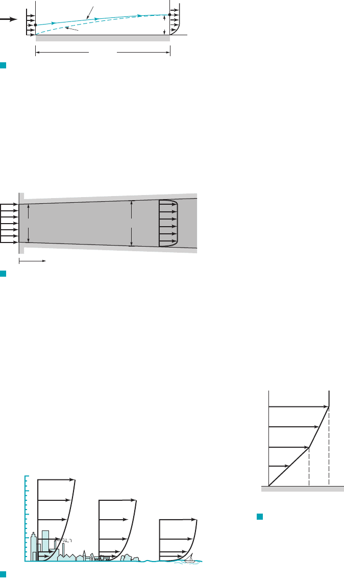
9.22 An atmospheric boundary layer is formed when the wind

blows over the earth’s surface. Typically, such velocity profiles

can be written as a power law: where the constants a and

n depend on the roughness of the terrain. As is indicated in Fig.

P9.22, typical values are for urban areas, for

woodland or suburban areas, and for flat open country

1Ref. 232. (a) If the velocity is 20 ft兾s at the bottom of the sail on

your boat what is the velocity at the top of the mast

(b) If the average velocity is 10 mph on the tenth1y  30 ft2?

1y  4 ft2,

n  0.16

n  0.28n  0.40

u  ay

U  0.5 m



b  4 m/  6 m

F I G U R E P9.30

___

*9.31 For a fluid of specific gravity flowing past a flat

plate with an upstream velocity of the wall shear stress

on a flat plate was determined to be as indicated in the table below.

Use the momentum integral equation to determine the boundary

U  5 m



SG  0.86

JWCL068_ch09_461-533.qxd 9/23/08 11:49 AM Page 526