Myron G. Best. Igneous and metamorphic 2003 Blackwell Science

Подождите немного. Документ загружается.

3.17 for the silica polymorphs). Other experimentalists

have used very ﬁnely pulverized mineral grains as

starting materials for experiments, but the surface and

strain energy imparted to the minute grains can over-

whelm the small Gs intrinsic to the phases. The nature

of sillimanite grains sometimes used as starting mater-

ial poses yet another difﬁculty. Other components, or

“impurities,” such as upwards of 1 wt.% of Fe

that

substitutes for Al

, inﬂuence the very small free

energy differences between sillimanite and the other

polymorphs. Consequently, reaction conditions and

equilibrium boundaries can be shifted by as much as a

few tens of degrees and stability ﬁeld boundaries

become narrow divariant bands in P–T space rather

than univariant lines. Minute, practically inseparable

intergrowths of quartz are common in some sillimanite,

further confusing stability relations.

In many rocks, sillimanite occurs not as isolated

single grains but rather as very ﬁne ﬁbrous bundles,

called ﬁbrolite, that are typically intimately intergrown

in muscovite or biotite (Figure 16.2). According to

Penn et al. (1999), the excess grain-boundary energy

of ﬁbrolite resulting from the small size of the ﬁbers,

together with the slight nonparallelism of neighboring

ﬁbers and possible Al–Si disordering in their lattice,

shifts the andalusite–sillimanite reaction by as much as

an estimated 140°C and the kyanite–sillimanite curve

by 30°C. Difﬁculty in nucleating an isolated grain

of sillimanite is overcome by nucleation on boundaries

of nonparallel mica ﬂakes during prograde metamor-

phism and the resulting ﬁbrolite mimics the misori-

ented ﬂakes.

SiO

Stability Diagram. Because of these kinetic

factors, widely discrepant univariant boundary lines

delineating polymorph stability ﬁelds have been deter-

mined by numerous experimentalists (Figure 16.3).

The set of univariant lines determined by Holdaway

and Mukhopadhyay (1993) is preferred by many

petrologists and is adopted here.

It is a useful exercise to recreate the Al

SiO

poly-

morph stability diagram from the thermodynamic data

provided by Holdaway and Mukhopadhyay (1993) and

presented here in Table 16.1. Qualitatively, kyanite,

having the smallest molar volume, ought to be stable

at highest P, whereas sillimanite ought to be stable

at highest T because its molar entropy is greatest.

An exact P–T point on the boundary lines between

polymorph stability ﬁelds can be calculated by com-

bining equations 3.1, 3.4, and 3.7 at constant P and T,

giving G H  TS. Here, the differentials dG

and dS in these equations have been replaced by the

change in free energy, G, in enthalpy, H, and in en-

tropy, S, for the polymorphic transition. At the equi-

librium T

between two coexisting polymorphs on

their corresponding boundary line at P  1 atm, G 

0 (Section 3.3); hence, H  T

S. Using values from

Table 16.1 we can solve for T

in the reaction kyanite

→ andalusite

The Clapeyron equation 3.13 in Section 3.3.1 can be

used to determine the slopes of the boundary lines.

Again, for the kyanite → andalusite transition

 11.84 bar/degree

This position and slope of the kyanite–andalusite equi-

librium line may be compared to those in Figure 16.3.

It is left as Problem 16.1 to determine the other two

boundary lines.

Application to Rocks. How reliable are polymorphs of

SiO

as mineral thermobarometers, indicating the

P–T conditions under which a particular polymorph

was stabilized? Even if experimental difﬁculties in the

determination of the stability diagram can be overcome,

and it can never be fully certain they have been, there



S

V



(91.60  82.86)J/K

(51.46  44.08)cm

 462 K  189°C



H

S



(2589.66  2593.70)kJ

(91.60  82.86)J/K

Metamorphic Mineral Reactions and Equilibria

477

0 0.2mm

Fibrolite

Biotite

Andalusite

16.2 Photomicrograph under plane-polarized light of ﬁbrolite in a

pelite hornfels near Lake Isabella, Sierra Nevada roof pendant,

California. Note that the ﬁbrolite is intimately intergrown with

biotite and does not replace nor lie in contact with andalusite.

remains the nagging question whether a particular

polymorph in a rock truly represents the most stable

phase at the time of metamorphism. Nature apparently

experiences the same kinetic difﬁculties as experiment-

alists do. Although many rocks contain just one poly-

morph, the presence of two polymorphs in one thin

section (such as andalusite and sillimanite, e.g. Fig-

ures 14.25d and 16.2) is not uncommon, and there are

reports of all three coexisting together.

In zoned terranes, univariant equilibrium prevails at

isograds; for example, at the sillimanite isograd where

kyanite reacts to form sillimanite. In ideal circum-

stances, the mineral equilibria between the polymorphs

can be frozen in the rock in a reaction texture. But the

widespread coexistence of two polymorphs throughout

part of a zoned terrane, where metamorphic conditions

just happened to fall on a univariant reaction boundary,

would seem to be improbable; the probability is indeed

remote that peak metamorphic conditions would fall

on the invariant triple point, preserving all three. It is

more possible that a polymorph nucleated metastably

or, more likely, persisted into the stability range of

another. Or a dissolved impurity component might

have created a divariant ﬁeld boundary wherein a

slight range in P–T conditions would stabilize two

polymorphs. Clearly, inferring P–T conditions from

SiO

polymorphs requires caution.

For polymorphs in other chemical systems, kinetics

appear to be less of a problem and they may be more

reliable mineral thermobarometers.

Although the univariant boundary lines and ther-

modynamic data of Holdaway and Mukhopadhyay

(1993) for the Al

SiO

polymorphs are preferred by

many petrologists, comparison of their stability ﬁeld of

478 Igneous and Metamorphic Petrology

P (kbar)

Depth (km)

0 200 400 600 800

Kyanite

Sillimanite

Andalusite

1000

T (°C)

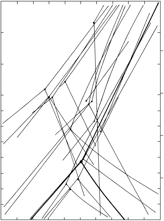
16.3 Al

SiO

stability diagram. Light lines are widely discrepant univariant boundary lines between stability ﬁelds of the polymorphs deter-

mined experimentally prior to 1969 by many investigators. Triple point where three boundary lines meet is emphasized by small ﬁlled

circle. Redrawn from Althaus (1969). The preferred phase diagram from Holdaway and Mukhopadhyay (1993) is indicated by heavy

lines. The triple point lies at 504  20°C and 3.75  0.25 kbar. Unlike the other two straight boundary lines, the andalusite–sillimanite

line is slightly curved, and three coordinates ﬁx its curvature: 500°C at 3.82 kbar, 600°C at 2.30 kbar, and 700°C at 0.95 kbar.

andalusite in Figure 16.3 with Figure 14.31 reveals an

apparent paradox. The solidus for a water-saturated,

minimum-T granite composition (Figure 5.24) lies at

a T well above the stability ﬁeld of andalusite. Yet

andalusite-bearing, peraluminous granites are well

known (Section 11.6.2), as are local migmatites and

pegmatites that contain this polymorph. The presence

of substantial concentrations of F and B might lower

the solidus T enough to stabilize andalusite in these

magmas; however, this is unlikely as the necessary

concentrations found by experiments are excessive for

natural systems. Alternatively, sillimanite might have

precipitated in the magma and then transformed into

more stable, lower-T andalusite during slow subsolidus

cooling. In yet other possibilities, andalusite might have

grown metastably above the solidus in the stability ﬁeld

of sillimanite, or some sort of subsolidus metasomatism

might have been involved, converting an alkali silicate

into andalusite (see Section 16.8.1).

16.4 NET TRANSFER SOLID–SOLID

REACTIONS

In discontinuous net transfer reactions, heterogeneous

mineral equilibria among multiple participating phases

can be represented by a written stoichiometric reaction

and by a P–T diagram that shows stability ﬁelds of

mineral assemblages and boundary lines between

them. We begin our discussion of net transfer reactions

using only pure solid phases, including ideal end-

members, where there is no solid solution.

16.4.1 Basic Relations in a System of Pure

End-Member Phases

Consider the equilibrium

16.1 Ca

 SiO

 CaAl

grossular quartz anorthite

 2CaSiO

wollastonite

in which the higher T and lower P assemblage is on the

right (Figure 16.4). LeChatelier’s principle (Section

3.3.1) tells us that this higher grade assemblage should

be the one of greater entropy and molar volume. Ther-

modynamic data in Table 16.2 conﬁrm that it is anor-

thite  2 wollastonite

Grs

 S

Qtz

 S

 2S

260.1  41.5  199.3  163.4

Grs

 V

Qtz

 V

 2V

12.528  2.269  10.079  7.98

These same entropy and volume data allow us to

quantify the slope (dP/dT) of the reaction boundary

line in P–T space. According to the Clapeyron

equation 3.13

Where this positive sloping line is positioned in P–T

space can be found in the same manner as the ﬁeld

boundary lines were determined above for the Al

SiO

polymorphs but using data in Table 16.2. Thus, the

equilibrium T

for reaction 16.1 at 1 atm is



61 J/K

3.262 J/bar

 18.7 bar/degree



(199.30  163.4)  (260.1  41.5)

(10.079  7.98)  (12.578  2.269)



S

V



 2S

)  (S

Grs

 S

Qtz

)

 2V

)  (V

Grs

 V

Qtz

)

Metamorphic Mineral Reactions and Equilibria

479

P (kbar)

3 Anorthite

Depth (km)

200 400 600 800 1000

Anorthite  2 wollastonite

Grossular  quartz

Albite  nepheline

2 Jadeite

Jadeite  quartz

Albite

Grossular



quartz



2 kyanite

1200

T (°C)

 498°C

 8858.6 bar at 25°C

16.4 Univariant discontinuous reaction boundary lines involving

albite and anorthite for pure phases based on laboratory

synthesis experiments. Redrawn from Hays (1967), Newton

and Fyfe (1976), and Koziol and Newton (1988). The dashed

line through P

and T

is based on calculations in text from

data in Robie and Hemingway (1995).

Table 16.2. Thermodynamic Data per Mole for

Some Pure Solid Phases at 25°C (298.15K) and 1 Bar

from Robie and Hemingway (1995)

V (J/

BAR

)* S ( J/K) H (

J) G (

Anorthite 10.079 199.3 4234.0 4007.9

Grossular 12.528 260.1 6640.0 6278.5

Wollastonite 3.990 81.7 1634.8 1549.0

Quartz 2.269 41.5 910.7 856.3

Coesite 2.064 38.5 907.8 852.5

*1 J/bar  10 cm

A second method of determining a point on the equi-

librium boundary line begins with an expression for

the free energy,  , of Reaction 16.1 at the equi-

librium T

and P

relative to some reference state,

G° , such as 25°C (298.15K) and 1 bar. We ﬁrst

integrate Equation 3.11, dG

SdT, at constant P,

and Equation 3.12, dG

 VdP, at constant T, between

the reference state and the equilibrium T

and P

and

then combine to give

16.2

S(T

 T

ref

)

This expression assumes that V is independent of P

and S of T. Here we note that, at the equilibrium T

and P

, 0; furthermore, the calculations

are simpliﬁed if we evaluate P

where T

 25°C 

ref

. Equation 16.2 becomes

16.3 

Using data in Table 16.2, V  3.262 J/bar and

G  28 900 J. Remembering that P

ref

 1 bar,

we can solve for P

, obtaining 8858.6 bar at 25°C.

Although this is a geologically unrealistic P, extrapola-

tion to higher P–T values along a properly sloping line

(18.7 bar/degree) is quite reasonable.

From the alternate reaction points at T

 498°C

and 1 atm and P

8858.6 bar at 25°C on the ﬁeld

boundary line determined by the two methods, a slop-

ing line can be plotted in Figure 16.4 by taking some

arbitrary “rise and run” of, say, (400  18.7) bar/400°C

 7480 bar/400°C. This line based on thermodynamic

data deviates increasingly at higher P from the bound-

ary line based independently on laboratory synthesis

experiments. One reason for the discrepancy is a P de-

pendence on the V of the reaction, which we ignored.

In many cases, different approaches yield signiﬁcantly

different results, forcing the petrologist to critically

examine the data, rejecting one or more or all sets, and

possibly performing additional experimental work to

try to resolve the discrepancies.

It may be noted that the boundary lines in Figure

16.4 are straight lines; that is, they are linear functions

of P and T. However, some solid–solid equilibria deﬁne

slightly curved lines where molar volumes and en-

tropies vary with respect to P and T; the andalusite–

sillimanite reaction line in Figure 16.3 is an example.

Using computer spreadsheets, it is easy to take into

account heat capacities, compressibilities, and so on to

ref

G

ref

V(P

 P

ref

)

G

G°

ref

V(P

 P

ref

)

ref



47 100 J

61.1 J/K

 771K  498°C



(4234 000 2{1634 800})  (6 640 000  910 700)

(199.30  163.4)  (260.1  41.5)



H

S

create more accurate reaction lines from thermody-

namic data (Nordstrom and Munoz, 1994, p.101).

It is important to note in Figure 16.4 that the stabil-

ity ﬁeld of a phase, or phase assemblage, shrinks in the

presence of an additional reacting phase. Thus, the P–T

stability ﬁeld of anorthite  wollastonite lies within,

and at lower P and T than, the ﬁeld of anorthite alone.

Where kyanite is present, grossular  quartz is stable

only at pressures higher than in systems lacking kyan-

ite. Albite encompasses the more restricted stability

ﬁeld of the assemblage albite  nepheline, and the

stability ﬁeld of jadeite  quartz is a part of the larger

ﬁeld of stable jadeite. This same concept explains why

olivine in basaltic systems is stable to only deep levels

of the continental crust (Figure 5.11), whereas in peri-

dotite it is stable to depths of a magnitude greater in

the mantle (Figure 1.3). In basaltic systems, olivine is

consumed in reactions with plagioclase at modest P,

whereas in peridotite olivine does not react with any of

the other coexisting phases. (Nonetheless, beginning

near 410 km depth in the mantle, olivine undergoes a

phase transformation into a denser spinel-like mineral.)

In the three component system SiO

–CaO–Al

the phase rule indicates that the boundary line repre-

sents a state of univariant equilibrium where all four

solid phases (grossular  quartz  anorthite  wollas-

tonite) coexist in equilibrium (F  2  C 2 

3  4  1). For P–T values off the univariant line, no

more than three phases can coexist stably in states of

divariant equilibrium where T and P can freely and

independently vary without affecting the phases in

equilibrium. Examination of reaction 16.1 indicates

which three phases can coexist. In the low-T divariant

ﬁeld, grossular and quartz occur stably together but

wollastonite or anorthite may also be present, but not

both. In the high-T divariant ﬁeld, wollastonite and

anorthite are stably coexistent but grossular or quartz

may also be present, but not both.

In most stability diagrams only the critical deter-

mining phases are indicated, such as the lower T

assemblage grossular  quartz and the higher T

assemblage wollastonite  anorthite in Figure 16.4. In

most instances, the molar proportions of grossular and

quartz would not be exactly the same in a rock under-

going prograde metamorphism at, say, 10 kbars and

900°C. So what happens is that the lesser of one of

these reactant phases, let’s say it is quartz, is entirely

consumed while the more abundant and excess grossu-

lar persists stably above 900°C, together with the prod-

uct phases wollastonite and anorthite. The reaction

at 10 kbar progresses at 900°C until quartz is entirely

consumed and only then can T increase in the heating

system, bringing it into the higher T divariant ﬁeld.

In the very unusual instance where the number of

moles of grossular is exactly equivalent to that of

quartz in a rock, an increase in T above 900°C at

480 Igneous and Metamorphic Petrology

10 kbars will result in the total consumption of both of

these two reactants into anorthite and wollastonite.

This product phase assemblage is divariant because it

consists of two components, CaSiO

and Al

SiO

Phase relations for the model reaction grossular 

quartz  anorthite  2 wollastonite are conveniently

depicted in a triangular composition, or compatibility,

diagram for the three components SiO

, CaO, and

that is drawn for a restricted range of P–T

conditions (Figure 16.5). Chemographic devices such

as this were described in Section 15.3. Stably coexisting

phases are connected by tie lines. At low T, the divari-

ant assemblage grossular  quartz is stable. A rock

whose proportions of components place it at point A

consists of only grossular and quartz in proportions

given by the lever rule. However, two three-phase

assemblages are also stable possibilities. In rock B,

an excess of Al

stabilizes anorthite in addition to

grossular  quartz whereas a deﬁciency in rock C sta-

bilizes wollastonite in addition to grossular  quartz.

At, say, 10 kbars an increase in T above 900°C (Figure

16.4) will result in a tie-line switching reaction in

which grossular  quartz react to form more stable

anorthite  wollastonite. As a result of this discontinu-

ous reaction, rock A now consists of equal proportions

of only anorthite  wollastonite, while in rocks B and

C the modal excess of quartz cannot be consumed in

the reaction, resulting in the three-phase assemblage

anorthite  wollastonite  quartz.

16.4.2 Model Reactions in the Basalt–Granulite–

Eclogite Transition

Metabasites are among the most common rocks in

regional metamorphic terranes in orogens. Signiﬁc-

ant changes in mineral assemblages in their maﬁc

protoliths reﬂect the effects of increasing pressures in

deepening parts of the mountain belt. In this section, to

simplify the nature of reactions during increasing P we

utilize model reactions between pure idealized end-

member phases, ignoring the widespread solid solution

that prevails in the rock-forming minerals.

Changing mineral equilibria in metabasites are

commonly recorded in corona and symplectite reaction

textures. Because of the commonly dry composition of

basaltic protoliths and possibly also because of limited

time, the sphere of effective diffusion is restricted

and recrystallization is commonly incomplete. Con-

sequently, a jacketing corona of more stable product

phases surrounds a destabilized reactant grain. In

Figure 16.6, more stable orthopyroxene (hypersthene)

crystallized at the contact between incompatible

olivine and plagioclase. Excess Mg and Fe from this

replacement diffused into the plagioclase where it

reacted to form spinel, and Ca from decomposing

plagioclase diffused in the opposite direction toward

the olivine, where diopside formed.

To a ﬁrst approximation, corona development in the

metagabbros in Figure 16.6 can be modeled by simple

reactions between pure end-member phases, ignoring

minor components. For the replacement of olivine by

orthopyroxene

16.4 2Mg

SiO

 2MgSiO

 2MgO

forsterite enstatite

and for the formation of the rim of diopside  spinel

surrounding the orthopyroxene

16.5 CaAl

 2MgO  CaMgSi

 MgAl

anorthite diopside spinel

Metamorphic Mineral Reactions and Equilibria

481

Wollastonite

Low T High TMole

proportions

Quartz

Anorthite

Grossular

CaO Al

SiO

16.5 Phase relations for the equilibrium 16.1 in terms of the components CaO–SiO

–Al

These two reactions can be added together to give

16.6 2Mg

SiO

 CaAl

forsterite anorthite

 2MgSiO

 CaMgSi

 MgAl

enstatite diopside spinel

Molar entropies and volumes for these assemblages at

25°C and 1 atm are listed in Robie and Hemingway

(1995) as follows:

(2FoAn)

 387.5 J/K

(2EnDiSpl)

 364.0 J/K

(2FoAn)

 188.09 cm

(2EnDiSpl)

 168.42 cm

If the relative values of these quantities do not change

at high P and T, they indicate that the assemblage

2Fo  An ought to be stable at higher T because of

its greater entropy compared to 2En  Di  Spl.

Similarly, it is stable at lower P because of its greater

volume. Therefore, because S/V is positive, the

Clapeyron Equation (3.3.1) indicates the univariant

boundary line for the reaction 2Fo  An  2En  Di 

Sp has a positive slope on a P–T diagram (Figure 16.7).

Because anorthite has a relatively large molar volume,

with increasing P it reacts with MgO (from breakdown

of olivine) forming a smaller volume (denser) assem-

blage of diopside  spinel according to reaction 16.6.

Al can be sequestered in high-P pyroxenes as the Mg-

and Ca-tschermak end-members (Special Interest Box

16.1). Tschermak end-members do not exist as distinct

pure minerals. In a reaction between plagioclase and

olivine, previously modeled by reaction 16.6, alternate

products would be aluminous pyroxene solid solutions

containing the tschermak end-members, as follows

16.7 3Mg

SiO

 4CaAl

forsterite anorthite

 2MgSiO

·MgAl(AlSi)O

Al-enstatite

 2CaMgSi

·CaAl(AlSi)O

 SiO

Al-clinopyroxene quartz

482 Igneous and Metamorphic Petrology

BASALT (Pl

 Cpx  Opx  Ol)

Crystals



melt

GRANULITE

Solidus

ECLOGITE

Al-Cpx

 Grt  Ky  Opx  Qtz (or Cs)

Low-P ~3–5 kbar



Cpx



Opx





Spl

Medium-P

Pl  Al

Cpx  Al

-Opx  Qtz

High-P ~10 kbar

Cpx  Grt  Pl  Qtz

16.8 – 16.10

16.9

16.7

16.6

16.7 Schematic stability ﬁelds of basaltic, granulitic, and eclogitic

mineral assemblages separated by model univariant reactions

16.6–16.10. Boundary line slopes are schematic and assumed

to be linear. Eclogite and granulite facies assemblages are

stable in either the crust or upper mantle depending upon T.

Minerals listed in approximate order of modal abundance.

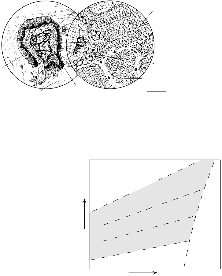
Plagioclase

Diopside

+ spinel

Hypersthene

Spinel

Diopside

Plagioclase with

minute spinel

inclusions

Relict

olivine

(a) (b)

0 0.3mm

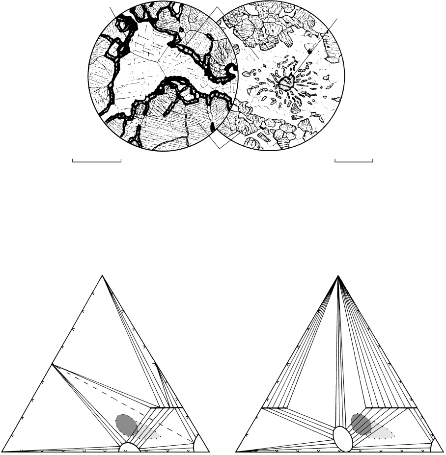
16.6 Corona reaction textures in metagabbros developed at original olivine–plagioclase grain contact. (a) Sample from Risor, southern

Norway, showing an inner corona of ﬁbrous orthopyroxene (hypersthene) that has replaced original olivine and surrounded by an

outer corona of a ﬁne intergrowth of diopside  spinel that has replaced plagioclase. (b) Sample from the Barton Garnet Mine, Gore

Mountain, New York. Corona of hypersthene and diopside that is texturally more stable than (a) because of coarser granoblastic grains.

Although a few small spinels (black) occur in the diopside aggregate, most of them cloud plagioclase grains and have grown preferen-

tially along twin planes and grain boundaries. Both reproduced with permission from Nockolds SR, Knox RWO’B, Chinner GA. 1978.

see Yardley et al. (1990, Figures 102–104).

The albite end-member in plagioclase has a smaller

molar volume than anorthite and, therefore, albitic

plagioclase is stable to higher P. But ultimately, it too

becomes unstable. Albite decomposes to form the

aluminous pyroxene, jadeite, NaAlSi

, according to

16.8 NaAlSi

 NaAlSi

 SiO

albite jadeite quartz

Jadeite is a naturally occurring phase, locally in vir-

tually pure form, in high P/T mineral assemblages

(Figure 16.4) of the eclogite and blueschist facies.

Jadeite is also a prominent end-member, along with

diopside (CaMgSi

) and other lesser components, in

omphacite (Appendix A). Ca–Mg–Fe–Al garnet and

omphacite are major constituents of eclogite together

with smaller amounts of other possible accessory min-

erals including kyanite, quartz (or coesite), orthopy-

roxene, rutile, phengite, paragonite, and epidote, but

never plagioclase. High-P omphacites can equilibrate

during decompression to a symplectitic intergrowth of

plagioclase in diopside (Figure 15.11).

Garnet is yet another dense repository for Al, Mg,

and Ca at high P. Anorthite can react with enstatite to

form garnet according to the reaction

16.9 CaAl

 2(Mg,Fe)SiO

anorthite orthopyroxene

 Ca(Mg,Fe)

 SiO

garnet quartz

Reaction textures resulting from the forward and

backward progress of this reaction are shown in Fig-

ure 16.8.

Another reaction consuming anorthite is

16.10 3CaAl

 Ca

anorthite grossular

 2Al

SiO

 SiO

kyanite quartz

where grossular is dissolved in garnet solid solutions.

The univariant line for this reaction is shown in Figure

16.4.

The reactions listed above serve as models for uni-

variant boundary lines in P–T space between ﬁelds

where basaltic, granulitic, and eclogitic mineral assem-

blages are stable (Figure 16.7). This ﬁgure is highly

schematic and no exact values are placed on the coor-

dinate axes because of the chemical variability of nat-

ural basaltic systems. Furthermore, reactions involving

solid solutions in rocks are at least divariant and are

thus “smeared” over P–T bands, in contrast to the uni-

variant lines indicated.

Further insights into the continuous mineralogical

transitions depicted in P–T space in Figure 16.7 are re-

vealed in ACF diagrams (described in Section 15.3.3)

that show solid solution of the compatible phases. In

unmetamorphosed basaltic and gabbroic rocks, the sta-

ble mineral assemblage is plagioclase  clinopyroxene

 Fe–Ti oxides  orthopyroxene  olivine (Figure

15.26). With increasing P under low volatile fugacities,

olivine ceases to be stable in the presence of calcic pla-

gioclase and is consumed by reaction 16.6. Low- to

mid-P granulite-facies metabasites consist of increas-

ingly more sodic plagioclase  aluminous clinopyrox-

ene  aluminous orthopyroxene. At higher P, garnet-

forming reactions 16.9 and 16.10 take place, causing a

tie-line switch to Fe–Mg–Ca–Al garnet  clinopyrox-

ene compatibility from the lower P plagioclase  or-

thopyroxene compatibility, changing the topology of

the the ACF diagram in Figure 16.9a. Recall that tie-

line switching is one diagrammatic manifestation of a

discontinuous reaction, in this case plagioclase  ortho-

pyroxene → garnet  clinopyroxene. Nonetheless,

plagioclase remains stable in more aluminous metaba-

sites but is absent in more maﬁc protoliths. At highest

P in the deep, thick continental crust or upper mantle,

further discontinuous reactions occur in metabasites,

creating plagioclase-free mineral assemblages of the

eclogite facies and causing further changes in conﬁgura-

tion of the compatibility diagram (Figure 16.9b). In

these highest P reactions, plagioclase is fully consumed

in what are called terminal disappearance reactions

because this phase is not stable in any rock composi-

tion. Dense garnets of a wider range of composition are

Metamorphic Mineral Reactions and Equilibria

483

Special Interest Box 16.1 Coordination of

oxygen around Al and Si in high-P minerals

At relatively low pressures, Al and Si cations are

tetrahedrally coordinated with oxygen anions in

aluminosilicate minerals but with increasing pres-

sures a more compact, lower molar volume octa-

hedral conﬁguration develops where six oxygens

surround a cation instead of four. This transition to

a denser packing and higher coordination begins

for Al in pyroxene end members at mid-crustal

pressures. In the Mg- and Ca-tschermak end-

members, MgAl

(Al

Si)O

andCaAl

(Al

Si)O

one Al has a tetrahedral coordination (IV) while the

other is octahedral (VI). In the jadeite end-member,

NaAl

, all of the Al is in six-fold coordination.

The only silica polymorph possessing octahedral

coordination is the densest one, stishovite (atmos-

pheric density 4.28 g/cm

compared to 2.65 g/cm

for -quartz). Stishovite is only stable at pressures

(Figure 5.1) well beyond those to which continental

sialic rocks are normally subjected but it has been

found in some meteorite impact rocks that were

subjected to extreme transient pressures in the

shock wave.

stabilized, together with the densest Al

SiO

poly-

morph, kyanite, in relatively aluminous protoliths.

Ca and Al sequestered in plagioclase at lower P are

lodged in garnet, while Na and Al, together with Ca,

Mg, and Fe, occur in solid solution in omphacite

clinopyroxene.

16.5 CONTINUOUS REACTIONS

BETWEEN CRYSTALLINE SOLID

SOLUTIONS

Because of extensive solid solution in almost all

metamorphic rock-forming minerals, most reactions,

484 Igneous and Metamorphic Petrology

01mm 0.50mm

Pyroxene

Plagioclase

Garnet

(a) (b)

16.8 Reaction textures in granulite-facies rocks modeled by reaction 16.9 anorthite  orthopyroxene  garnet  quartz. (a) Sample of a

deep crustal inclusion in a kimberlitic pipe, Delegate, New South Wales, Australia. Well developed crystalloblastic fabric has been

modiﬁed by growth of more stable garnet (black borders) along boundaries between incompatible orthopyroxene and plagioclase grains.

(b) Sample from the Granulitgeberge, Hartmannsdorff, Sachsen, Germany. The same reaction in reverse has produced a symplectite

(vermicular (“wormy”) intergrowth) of orthopyroxene  plagioclase from garnet, only a small remnant of which remains. Both repro-

duced with permission from Nockolds SR, Knox RWO’B, Chinner GA. 1978. Petrology for students. New York, Cambridge University Press.

(a) A

Kyanite

GRANULITE

FACIES

 magnetite

 ilmenite

Spinel

Garnet

Plagioclase

Calcite

OrthopyroxeneClinopyroxene

(b) A

Kyanite

ECLOGITE

FACIES

 rutile

 quartz

(or coesite)

Garnet

Grossular

Calcite

OrthopyroxeneOmphacite

16.9 ACF diagrams showing the transition between mineral assemblages in metabasites of the granulite facies and eclogite facies. Most basalts

and gabbros plot in the dark shaded area but some more maﬁc ones, such as picrite, fall in the lighter shaded area. Compare the

assemblage in basaltic protoliths in Figure 15.26. (a) Dashed tie-line represents compatibility (stable coexistence) of plagioclase 

aluminous orthopyroxene in mid-P granulites. At higher P, the anorthite molecule in plagioclase reacts with orthopyroxene to form

garnet as in reaction 16.9. Remaining plagioclase in less maﬁc metabasites is more sodic and coexists with garnet and Al-rich clinopy-

roxene. In the eclogite facies (b), plagioclase is not stable and most metabasites consist of a Ca–Fe–Mg–Al garnet solid solution

plus Ca–Fe–Mg–Na–Al omphacitic clinopyroxene (Appendix A, 13) together with accessory rutile. Kyanite appears in more Al-rich

eclogites, orthopyroxene in more maﬁc ones, while quartz (coesite at higher pressures, Figure 5.11) may be stabilized in more silica-rich

eclogites.

including those just discussed for metabasites, take

place over a range of changing P and T in which both

reactant and product phases coexist. In such contin-

uous mineral reactions both modal proportions and

chemical compositions of reactant and product solid

solutions change until the reactant, or reactants, is

entirely consumed, terminating the reaction.

16.5.1 Solid Solution in the Continuous Net

Transfer Reaction Plagioclase  Jadeitic Clinopyroxene

 Quartz

The discontinuous reaction involving pure phases

albite  jadeite  quartz was shown above in Figure

16.4 and equation 16.8. This equilibrium is applicable

to high P/T rocks of the blueschist facies where, how-

ever, the widespread presence in the rocks of Ca, Mg,

and Fe leads to solid solution of these components in

the plagioclase and clinopyroxene. Accordingly, a little

anorthite is dissolved in the plagioclase and typically

greater concentrations of diopside and aegirine in

clinopyroxene resulting from Ca–Mg b Na–Al and

3

b Al substitutions, respectively. Because of the

complexity of the solid solutions, exact balanced stoi-

chiometric equations are impossible to write where

Ca–Al substitutes in plagioclase and Ca–Mg–Fe in

clinopyroxene; hence, there are many degrees of com-

positional freedom, guaranteeing continuous reactions

where all three phases coexist stably over a range of P

and T. The compositional variability and dilution of

the jadeite end-member results in a shift of the equilib-

rium in P–T space, extending the stability ﬁeld of the

less pure clinopyroxene in the presence of quartz

to lower pressures. Hence, this equilibrium has the

potential of serving as a geobarometer.

The extent of the shift can, in principle, be calcu-

lated using thermodynamic tools and data tied wher-

ever possible to experimental data. For reaction 16.8

where all phases are pure the univariant reaction line is

governed by the relation

16.11 G  G

 G

Qtz

– G

 0

But where there is solid solution in the plagioclase and

especially the clinopyroxene the condition for equilib-

rium is (Section 3.5)

16.12 G 

16.13 G  RT lnK

where G is the calculated change in free energy

(equation 16.8) for pure phases at the P and T of inter-

est and K

is the equilibrium constant

16.14 K



The activities (thermodynamically effective concen-

trations) of jadeite, NaAlSi

, in clinopyroxene and

NaAlSi

Cpx

·a

SiO

Qtz

NaAlSi



NaAlSi

Cpx



Qtz

SiO



NaAlSi

 0

albite, NaAlSi

, in plagioclase must then be evaluated.

(The activity of silica in quartz, a  1.) Although

the chemical compositions of the stably coexisting pla-

gioclase and clinopyroxene in the mineral assemblage

of a blueschist are readily and accurately determined

by electron microprobe analyses, determination of activ-

ities from measured compositions requires a suitable

model relationship. Several theoretical models are in

use (Spear, 1993, pp. 176–205) depending on the ex-

tent to which the constituent ions in speciﬁc crystallo-

graphic sites interact with one another in the natural

solid solution. Which model to apply depends on the

desired rigor and how well it ﬁts independent infor-

mation obtained from experiments. Simply equating

activity with measured concentration generally yields

inaccurate results.

Results of experiments by Holland (1983) on the

equilibria plagioclase  jadeitic clinopyroxene  quartz

are summarized in Figure 16.10. For clinopyroxenes

with about 0.8 mole fraction of the jadeite end-member

that coexist with quartz the equilibrium P is depressed

about 1 kbar from that for pure jadeite. Decreasing P

signiﬁcantly reduces the equilibrium concentration of

the jadeite end-member.

16.5.2 Continuous Exchange Reactions in Fe–Mg

Solid Solutions

We now deal with a more common type of continuous

reaction that involves Fe–Mg substitution in many maﬁc

rock-forming minerals. Similar continuous reactions

SiO

Qtz

Metamorphic Mineral Reactions and Equilibria

485

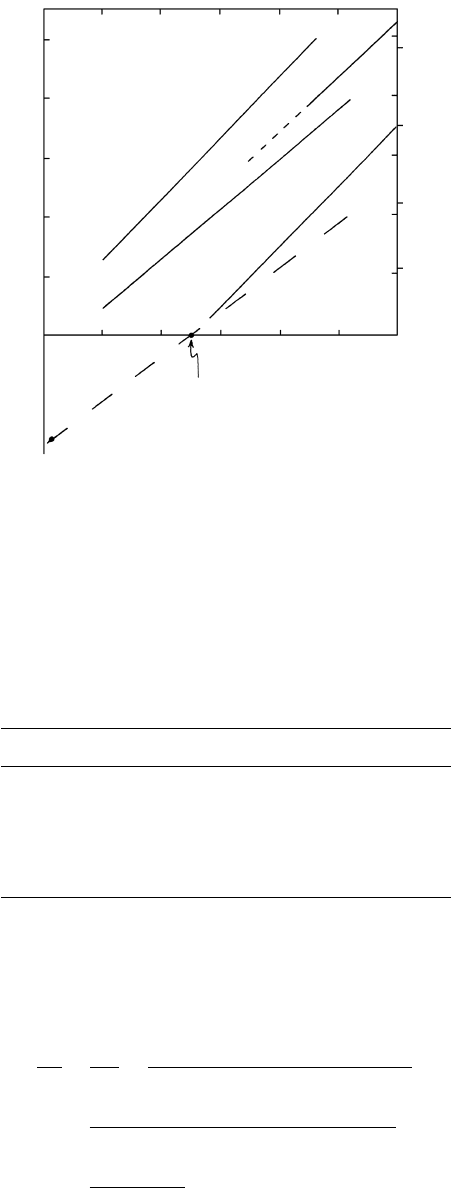
P (kbar)

Depth (km)

200 12001000800600400

T (°C)

Jadeite  quartz

Albite

0.2

0 5

0 8

1 0

Clinopyroxene 

quartz  plagioclase

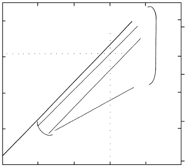
16.10 Clinopyroxene  plagioclase  quartz equilibria. Heavy line

is for the univariant discontinuous reaction involving the pure

end members (compare Figure 16.4). Light lines are for equi-

libria involving jadeite–diopside solid solutions (0.8, 0.5, and

0.2 mol fractions of jadeite) with coexisting quartz and sodic

plagioclase. Decreasing purity of jadeite corresponds to de-

creasing equilibrium P. At 800°C and 20.5 kbar, for example,

in an assemblage of quartz  plagioclase  clinopyroxene the

equilibrium composition of the latter phase would be

. Redrawn from Holland (1983).

occur in micas, amphiboles, and feldspars where

there are substitutions among Na, K, and Ca. Clearly,

continuous reactions are of particular signiﬁcance in

metamorphic rocks.

In contrast to the univariant polymorphic trans-

itions and discontinuous reactions that result in sharp

isograds in the ﬁeld, continuous reactions occur over

broad geographic domains in metamorphic terranes

but an isograd line can nonetheless be positioned at the

ﬁrst appearance of a solid solution, such as Fe–Mg–Ca

garnet. In compatibility diagrams, continuous reactions

cause continuously changing topologies manifest in

shifts and sweeps in tie-line orientations and conﬁgura-

tions that accompany expansions and contractions of

stability ﬁelds.

Because of differing crystal lattices, different miner-

als have different preferences for Fe and Mg. Con-

sequently, the mole fraction of the Mg end-member, or

the mole ratio Mg/(Mg  Fe

2

)  X

, will differ in

stably coexisting maﬁc minerals in a rock. In pelitic

rocks, ﬁve maﬁc minerals are common, including

garnet, staurolite, biotite, chlorite, and cordierite. The

relative partitioning of Fe and Mg is

16.15 X

Although X

is different for each stably coexsiting

mineral, the ratio by which Mg and Fe are partitioned

between any two minerals is essentially constant under

the same metamorphic conditions regardless of bulk

rock composition. Hence, garnet and biotite in Fe-rich

pelites will contain more Fe than these same phases in

Mg-rich rocks but the distribution ratio, or distribu-

tion coefﬁcient, K

, is constant for a given P and T.

Grt

6 X

Chl

6 X

Crd

486 Igneous and Metamorphic Petrology

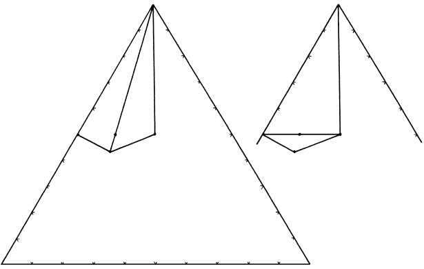
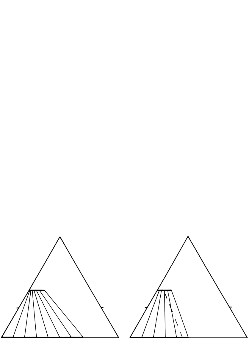
Biotite

FeO MgO

Garnet

 0.14

500°C

Biotite

FeO MgO

Garnet

 0.30

800°C

16.11 Contrast in the distribution coefﬁcient, K

, for Fe and Mg between stably coexisting garnet and biotite at two temperatures depicted

in AFM projections (Section 15.3.3). In the 800°C diagram, a representative tie-line from the 500°C plot is shown as a dashed line to em-

phasize that crossing tie-lines imply contrasting conditions (temperatures) of equilibration of coexisting phases. Redrawn from Spear

(1993).

(Compare K

with the partition coefﬁcient in magmatic

systems, Section 2.5.1). For the garnet–biotite pair

16.16 K

This distribution is displayed in Figure 16.11, where it

can be seen that for any Mg/Fe ratio in biotite the

ratio in a coexisting garnet is smaller so that K

 1.

Continuous reactions in maﬁc phases are con-

veniently broken down into Fe and Mg end-members.

A reaction of this type that is of considerable signiﬁc-

ance in low-grade pelitic rocks of regional Barrovian

zones can be expressed for Fe end-members as

16.17 Fe-chlorite  quartz  muscovite

 almandine  annite  water.

(It may be disconcerting that we are introducing a con-

tinuous reaction that also involves a ﬂuid, which has

not been discussed yet. However, such continuous

solid–ﬂuid reactions are very common and, for the pur-

poses of this section, the presence of water can simply

be ignored.) This reaction, which also happens to be of

the net transfer type, is univariant because there are

ﬁve components (K

O, FeO, Al

, SiO

, and H

and six phases, F  2  5  6  1. With addition of

another component, MgO, to the reaction system, it

becomes divariant and the general continuous reaction

is written as

16.18 chlorite  quartz  muscovite

 garnet  biotite  water.

Grt–Bt



(Mg/Fe)

Grt

(Mg/Fe)