Neubauer A., Freudenberger J., Kuhn V. Coding theory: algorithms, architectures and applications
Подождите немного. Документ загружается.

276 SPACE–TIME CODES
Original V-BLAST detector
r
w
1
ˆs
1
h
1
r
1
w
2
ˆs
2
h
2
r
2
w
3
ˆs
3
h
3
■ Zero Forcing (ZF) filter matrix equals Moore–Penrose inverse
W
ZF
= H
†
= H
H
H
H
−1
(5.103)
■ Error covariance matrices
ZF
= E
(W
H
ZF
r − x)(W
H
ZF
r − x)
H
= σ
2
N
· W
H
ZF
W
ZF
(5.104)
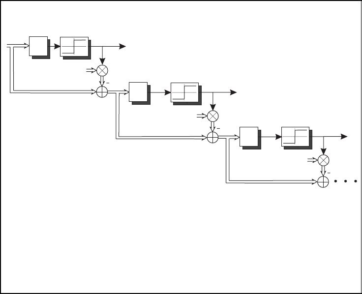
Figure 5.44: Structure of V-BLAST detector (Foschini, 1996; Foschini and Gans, 1998)
with Zero Forcing (ZF) interference suppression
elements determine the squared Euclidean distances between the separated layers and the
true symbols and equal the squared column norm of W
ZF
. Therefore, it suffices to deter-
mine W
ZF
; an explicit calculation of
ZF
is not required. We have to start with the layer
that corresponds to the smallest column norm in W
ZF
. This leads to the algorithm presented
in Figure 5.45.
The choice of the layer to be detected next in step 2 ensures that the risk of error
propagation is minimised. Assuming that the detection in step 4 delivers the correct symbol
ˆs
λ
ν
, the cancellation step 5 reduces the interference so that subsequent layers can be detected
more reliably. Layers that have already been cancelled need not be suppressed by the ZF
filter any more. Hence, the filter has more degrees of freedom and exploits more diversity
(K
¨
uhn, 2006). Mathematically, this behaviour is achieved by removing columns from H
which increases the null space for linear interference suppression.
In order to determine the linear filters in the different detection steps, the system matrices
describing the reduced systems have to be inverted. This causes high implementation costs.
However, a much more convenient way exists that avoids multiple matrix inversions. This
approach leads to identical results and is presented in the next section.

SPACE–TIME CODES 277
ZF-V-BLAST detection algorithm
■ Initialisation: set r
1
= r, H
1
= H
■ The following steps are repeated for ν = 1, ... , N
T
until all layers have
been detected:
1. Calculate the ZF filter matrix W
ZF
= H
†
ν
.
2. Determine the filter w
ν
as the column in W
ZF
with the smallest squared
norm, e.g. the λ
ν
th column.
3. Use w
ν
to extract the λ
ν
th layer by
˜s
λ
ν
= w
H
ν
· r
ν
.
4. Detect the interference-free layer either by soft or hard decision
ˆs
λ
ν
= Q
S
(˜s
λ
ν
).
5. Subtract the decided symbol ˆs
λ
ν
from r
ν
r
ν+1
= r
ν
− h
λ
ν
ˆs
λ
ν
and delete the λ
ν
th column from H
ν
, yielding H
ν+1
.
Figure 5.45: V-BLAST detection algorithm (Foschini, 1996; Foschini and Gans, 1998)
with Zero Forcing (ZF) interference suppression
MMSE Extension of V-BLAST
As mentioned above, the perfect interference suppression of the ZF filter comes at the
expense of a severe noise amplification. Especially at low signal-to-noise ratios, it may
happen that the ZF filter performs even worse than the simple matched filter. The noise
amplification can be avoided by using the MMSE filter derived on page 274. It provides
the smallest mean-squared error and represents a compromise between residual interfer-
ence power that cannot be suppressed and noise power. Asymptotically, the MMSE filter
approaches the matched filter for very low SNRs, and the ZF filter for very high SNRs.
From the optimisation approach
W
MMSE
= argmin
W∈C
N
T
×N
R
E
4
4
W
H
r − s
4
4
2
we easily obtain the MMSE solution presented in Equation (5.105) in Figure 5.46. A con-
venient way to apply the MMSE filter to the BLAST detection problem without new
derivation is provided in Equation (5.106). Extending the channel matrix H in the way
278 SPACE–TIME CODES
MMSE extension of V-BLAST detection
■ Minimum Mean-Square Error (MMSE) filter matrix
W
MMSE
= H
H
H
H +
σ
2
N
σ
2
N
I
N
T
−1
(5.105)
■ Relationship between ZF and MMSE filter
W
MMSE
(H) = W
ZF
(H) with H =
H
σ
N
σ
X
I
N
T
(5.106)
■ Error covariance matrices
MMSE
= E
(W
MMSE
r − x)(W
MMSE
r − x)
H
= σ
2
N
·
H
H
H +
σ
2
N
σ
2
N
I
N
T
−1
(5.107)
Figure 5.46: Procedure of V-BLAST detection (Foschini, 1996; Foschini and Gans,
1998) with Minimum Mean-Square Error (MMSE) interference suppression
presented yields the relation
H
H
H =
H
H
σ
N
σ
X
I
N
T
·
H
σ
N
σ
X
I
N
T
=
H
H
H +
σ
2
N
σ
2
X
I
N
T
.
Obviously, applying the ZF solution to the extended matrix H
delivers the MMSE solution
of the original matrix H (Hassibi, 2000). Hence, the procedure described on page 275 can
also be applied to the MMSE-BLAST detection. There is only a slight difference that has
to be emphasised. The error covariance matrix
MMSE
given in Equation (5.107) cannot
be expressed by the product of the MMSE filter W
MMSE
and its Hermitian. Hence, the
squared column norm of W
MMSE
is not an appropriate measure to determine the optimum
detection order. Instead, the error covariance matrix has to be explicitly determined.
5.5.5 QL Decomposition and Interference Cancellation
The last subsection made obvious that multiple matrix inversions have to be calculated,
one for each detection step. Although the size of the channel matrix is reduced in each
detection step, this procedure is computationally demanding. K
¨
uhn proposed a different
implementation (K
¨
uhn, 2006). It is based on the QL decomposition of H, the complexity
of which is identical to a matrix inversion. Since it has to be computed only once, it
SPACE–TIME CODES 279
saves valuable computational resources. The QR decomposition of H is often used in the
literature (W
¨
ubben et al., 2001).
ZF-QL Decomposition by Modified Gram–Schmidt Procedure
We start with the derivation of the QL decomposition for the zero-forcing solution. An
extension to the MMSE solution will be presented on page 284. In order to illuminate the
basic principle of the QL decomposition, we will consider the modified Gram–Schmidt
algorithm (Golub and van Loan, 1996). Nevertheless, different algorithms that are based
on Householder reflections or Givens rotations (see Appendix B) may exhibit a better
behaviour concerning numerical robustness. Basically, the QL decomposition decomposes
an N
R
× N
T
matrix H = QL into an N
R
× N
T
matrix
Q =
q
1
··· q
N
T
−1
q
N
T
and a lower triangular N
T
× N
T
matrix
L =
L
1,1
L
2,1
L
2,2
.
.
.
.
.
.
L
N
T
,1
··· L
N
T
,N
T
.
For N
T
≤ N
R
, which is generally true, we can imagine that the columns in H span an N
T
-
dimensional subspace from C
N
R
. The columns in Q span exactly the same subspace and
represent an orthogonal basis. They are determined successively from µ = N
T
to µ = 1,
as described by the pseudocode in Figure 5.47.
First, the matrices L and Q are initialised with the all-zero matrix and the channel
matrix H respectively. In the first step, the vector q
N
T
is chosen such that it points in the
direction of h
N
T
(remember the initialisation). After its normalisation to unit length by
L
N
T
,N
T
=h
N
T
⇒q
N
T
= h
N
T
/L
N
T
,N
T
,
the projections of all remaining vectors q
ν<N
T
onto q
N
T
are subtracted from q
ν<N
T
. The
resulting vectors
q
ν
− L
N
T
,ν
q
N
T
point in directions that are perpendicular to q
N
T
and build the basis for the next step. Con-
tinuing with q
N
T
−1
, the procedure is repeated down to q
1
. The projection and subtraction
ensure that the remaining vectors q
1
to q
µ
are perpendicular to the hyperplane spanned by
the already fixed vectors q
µ+1
to q
N
T
. Hence, the columns of Q are mutually orthogonal.
After N
T
steps, Q and L are totally determined.
Successive Interference Cancellation (SIC)
Inserting the QL decomposition into our system model yields
r = QLx + n (5.108)

280 SPACE–TIME CODES
Modified Gram–Schmidt algorithm
■ Columns q
µ
of Q are determined from right to left.
■ Elements of triangular matrix L are determined from lower right corner to
upper left corner
Step Task
(1) Initialisation: L = 0, Q = H
(2) for µ = N
T
, ..., 1
(3) set diagonal element L
µ,µ
=q
µ
(4) normalise q
µ
= q
µ
/L
µ,µ
to unit length
(5) for ν = 1, ..., µ− 1
(6) calculate projections L
µ,ν
= q
H
µ
· q
ν
(7) q
ν
= q
ν
− L
µ,ν
· q
µ
(8) end
(9) end
Figure 5.47: Pseudocode of modified Gram–Schmidt algorithm for QL decomposition of
channel matrix H (Golub and van Loan, 1996)
The advantage of this representation becomes obvious when it is multiplied from the left-
hand side by Q
H
. On account of the to orthogonal columns in Q, Q
H
Q = I
N
T
holds and
the multiplication results in
y = Q
H
· r = Lx + Q
H
n =
L
1,1
0
L
2,1
L
2,2
0
.
.
.
.
.
.
.
.
.
L
N
T
,1
L
N
T
,2
··· L
N
T
,N
T
· x +
˜
n (5.109)
The modified noise vector
˜
n still represents white Gaussian noise because Q consists
of orthogonal columns. However, the most important property is the triangular structure
of L. Multiplication with Q
H
suppresses the interference partly, i.e. x
1
is totally free of
interference, x
2
only suffers from x
1
, x
3
from x
1
and x
2
and so on. This property allows a
successive detection strategy as depicted in Figure 5.48. It starts with the first layer, whose
received sample of which
y
1
= L
1,1
x
1
+˜n
1
can be characterised the signal-to-noise ratio γ
1
= L
2
1,1
E
s
/N
0
. After appropriate scaling, a
hard decision Q(·) delivers the estimate
ˆs
1
= Q
L
−1
1,1
· y
1
(5.110)
SPACE–TIME CODES 281
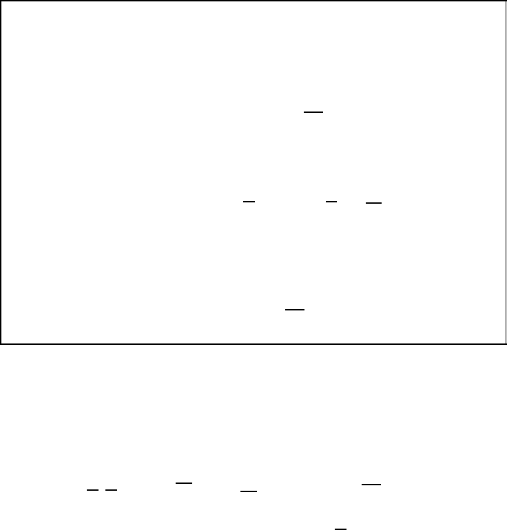
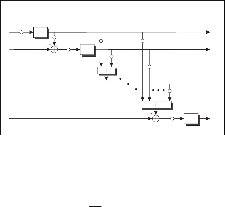
Successive interference cancellation
y
1
y
2
y
N
T
1/L
4,4
1/L
2,2
L
N
T
,N
T
−1
L
N
T
,2
L
3,2
L
N
T
,1
L
3,1
L
2,1
1/L
1,1
ˆs
1
ˆs
2
ˆs
N
T
Q(·)
Q(·)
Q(·)
Figure 5.48: Illustration of interference cancellation after multiplying r with Q
H
.
Reproduced by permission of John Wiley & Sons, Ltd
The obtained estimate can be used to remove the interference in the second layer which is
then only perturbed by noise. Generally ,the µth estimate is obtained by
ˆs
µ
= Q
1
L
µ,µ
·
5
y
µ
−
µ−1
ν=1
L
µ,ν
·ˆs
ν
6
(5.111)
Supposing that previous decisions have been correct, the signal-to-noise ratio amounts to
γ
µ
= L
2
µ,µ
E
s
/N
0
. This entire procedure consists of the QL decomposition and a subse-
quent successive interference cancellation and is therefore termed ‘QL-SIC’. Obviously,
the matrix inversions of the original BLAST detection have been circumvented, and only
a single QL decomposition has to be performed.
Optimum Post-Sorting Algorithm
Although the QL-SIC approach described above is an efficient way to suppress and cancel
interference, it does not take into account the risk of error propagation. So far, the algorithm
has simply started with the column on the right-hand side of H and continued to the left-
hand side. Hence, the corresponding signal-to-noise ratios that each layer experiences are
ordered randomly, and it might happen that the first layer to be detected is the worst one.
Intuitively, we would like to start with the layer having the largest SNR. Assuming perfect
interference cancellation, the layer-specific SNRs should decrease monotonically from the
first to the last layer.
282 SPACE–TIME CODES
From the last subsection describing the ZF-BLAST algorithm we know that the most
reliable estimate is obtained for that layer with the smallest noise amplification. Interlayer
interference does not matter because it is perfectly suppressed. This layer corresponds to
the smallest diagonal element of the error covariance matrix defined in Equation (5.104).
Applying the QL decomposition, the error covariance matrix becomes
ZF
= σ
2
N
· W
H
ZF
W
ZF
= σ
2
N
·
H
H
H
−1
= σ
2
N
· L
−1
L
−H
.
Obviously, the smallest diagonal element of
ZF
corresponds to the smallest row norm of
L
−1
. Therefore, we have to exchange the rows of L
−1
such that their row norms increase
from top to bottom. Unfortunately, exchanging rows in L or L
−1
destroys its triangular
structure. A solution to this dilemma is presented elsewhere (Hassibi, 2000) and is termed
the Post-Sorting Algorithm (PSA).
After the conventional unsorted QL decomposition of H as described above, the inverse
of L
−1
has to be determined. According to Figure 5.49, the row of L
−1
with the smallest
norm is moved to the top of the matrix. This step can be described mathematically by the
permutation matrix
P
1
=
0010
0100
1000
0001
.
Since the first row should consist of only one non-zero element, Householder reflections or
Givens rotations (Golub and van Loan, 1996) can be used to retrieve the triangular shape
again. They are briefly described in Appendix B. In this book, we confine ourselves to
Householder reflections denoted by unitary matrices
µ
. The multiplication of P
1
L
−1
with
1
forces all elements of the first rows except the first one to zero without changing the
row norm. Hence, the norm is now concentrated in a single non-zero element.
Now, the first row of the intermediate matrix P
1
L
−1
1
already has its final shape.
Assuming a correct decision of the first layer in the Successive Interference Cancellation
(SIC) procedure, x
1
does not influence other layers any more. Therefore, the next recursion
is restricted to a 3 ×3 submatrix corresponding to the remaining three layers. Although the
row norms to be compared are only taken from this submatrix, permutation and Householder
matrices are constructed for the original size. We obtain the permutation matrix
P
2
=
1000
0001
0100
0010
and the Householder matrix
2
. With the same argumentation as above, the relevant matrix
is reduced again to a 2 × 2 matrix for which we obtain
P
3
=
1000
0100
0001
0010
and
3
. The optimised inverse matrix has the form
L
−1
opt
= P
N
T
−1
···P
1
L
−1
·
1
···
N
T
−1
(5.112)
SPACE–TIME CODES 283
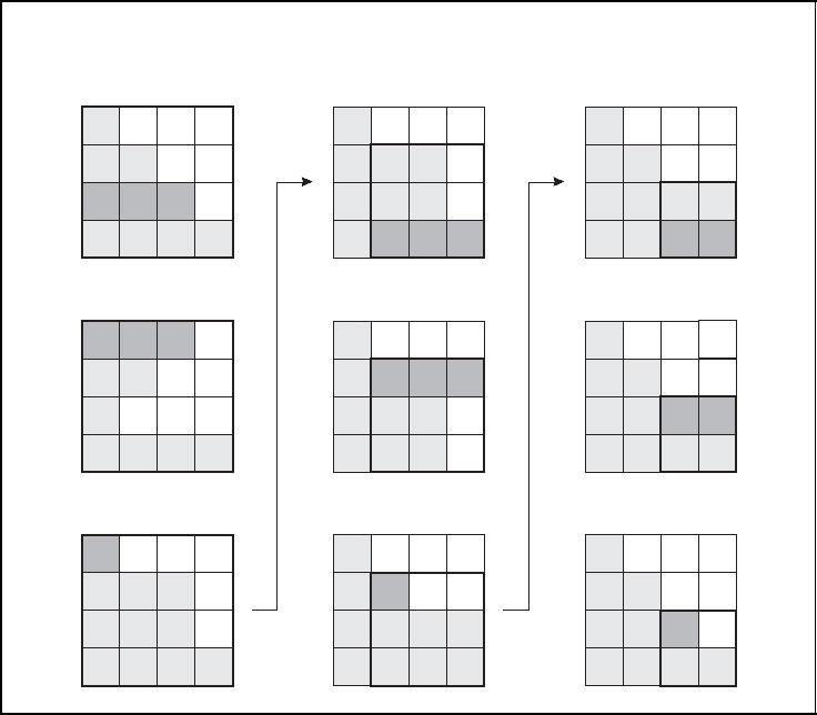
Optimum post-sorting algorithm
L
−1
P
1
L
−1
P
1
L
−1
1
P
1
L
−1
1
P
2
P
1
L
−1
1
P
2
P
1
L
−1
1
2
P
2
P
1
L
−1
1
2
P
3
P
2
P
1
L
−1
1
2
P
3
P
2
P
1
L
−1
1
2
3
Figure 5.49: Illustration of the post-sorting algorithm (white squares indicate zeros,
light-grey squares indicate non-zero elements, dark-grey squares indicate a row with a
minimum norm) (K
¨
uhn, 2006). Reproduced by permission of John Wiley & Sons, Ltd
Since all permutation and Householder matrices are unitary with PP
H
= P
H
P = I, we obtain
the final triangular matrix
L
opt
=
H
N
T
−1
···
H
1
· L · P
H
1
···P
H
N
T
−1
(5.113)
At most N
T
− 1, permutations and Householder reflections have to be carried out. The
optimised triangular matrix results in the QL decomposition of a modified channel matrix
H = QL ⇒ H
opt
= H · P
H
1
···P
H
N
T
−1
= Q
opt
L
opt
(5.114)
with
Q
opt
= Q ·
1
···
N
T
−1
(5.115)
Applying this result to the received vector r delivers
r = H · x + n = H
opt
· x
opt
+ n = H · P
H
1
···P
H
N
T
−1
· x
opt
+ n (5.116)
284 SPACE–TIME CODES
It follows that the optimised vector x
opt
equals
x = P
H
1
···P
H
N
T
−1
· x
opt
(5.117)
Hence, we can conclude that a QL decomposition of H with a subsequent post-sorting algo-
rithm delivers two matrices Q
opt
and L
opt
with which successive interference cancellation
can be performed. The estimated vector
ˆ
x
opt
has then to be reordered by Equation (5.117)
in order to get the estimate
ˆ
x.
MMSE-QL Decomposition
From Subsection 5.5.4 we saw that the linear MMSE detector is obtained by applying the
zero-forcing solution to the extended channel matrix
H
=
H
σ
N
σ
X
I
N
T
.
Therefore, it is self-evident to decompose H
instead of H in order to obtain a QL decom-
position in the MMSE sense (B
¨
ohnke et al., 2003; W
¨
ubben et al., 2003). The basic steps
MMSE extension of QL decomposition
■ QL decomposition of extended channel matrix
H
=
H
σ
N
σ
X
· I
N
T
= Q
· L =
Q
1
Q
2
· L
=
Q
1
· L
Q
2
· L
(5.118)
■ Error covariance matrix
MMSE
=
ZF
= σ
2
N
·
H
H
H
−1
= σ
2
N
· L
−1
L
−H
(5.119)
■ Inverse of L as byproduct obtained
σ
N
σ
X
· I
N
T
= Q
2
· L ⇒ L
−1
=
σ
X
σ
N
· Q
2
, (5.120)
■ Received vector after filtering with Q
H
y = Q
H
· r =
Q
H
1
Q
H
2
·
r
0
N
T
×1
= Q
H
1
· Hx + Q
H
1
· n (5.121a)
= L
· x −
σ
N
σ
X
· Q
H
2
x + Q
H
1
n (5.121b)
Figure 5.50: Summary of MMSE extension of QL decomposition

SPACE–TIME CODES 285
are summarised in Figure 5.50. The QL decomposition presented in Equation (5.118) now
delivers a unitary (N
R
+ N
T
) × N
T
matrix Q and a lower triangular N
T
× N
T
matrix L.
Certainly, Q
and L are not identical with Q and L, e.g. Q has N
T
more rows than the
original matrix Q. It can be split into the submatrices Q
1
and Q
2
such that Q
1
has the
same size as Q for the ZF approach.
Similarly to the V-BLAST algorithm, the order of detection has to be determined
with respect to the error covariance matrix given in Equation (5.119). Please note that
underlined vectors and matrices are associated with the extended system model. Since the
only difference between ZF and MMSE is the use of H
instead of H, it is not surprising
that the row norm of the inverse extended triangular matrix L
determines the optimum
sorting. However, in contrast to the ZF case, L
need not be explicitly inverted. Looking at
Equation (5.118), we recognise that the lower part of the equation delivers the relation given
in Equation (5.120). Hence, L
−1
is gained as a byproduct of the initial QL decomposition
and the optimum post-sorting algorithm exploits the row norms of Q
2
. This compensates
for the higher computational costs due to QL decomposing a larger matrix H
.
Since the MMSE approach represents a compromise between matched and zero-forcing
filters, residual interference remains in its outputs. This effect will now be considered in
more detail. Using the extended channel matrix requires modification of the received vector
r as well. An appropriate way is to append N
T
zeros. The detection starts by multiplying r
with Q
H
, yielding the result in Equation (5.121a). In fact, only a multiplication with Q
H
1
,is
performed, having the same complexity as filtering with Q
H
for the zero-forcing solution.
However, in contrast to Q and Q
, Q
1
does not contain orthogonal columns because it
consists of only the first N
R
rows of Q. Hence, the noise term Q
H
1
n is coloured, i.e. its
samples are correlated and a symbol-by-symbol detection as considered here is suboptimum.
Furthermore, the product Q
1
Q does not equal the identity matrix any more. In order
to illuminate the consequence, we will take a deeper look at the product of the extended
matrices Q
and H. Inserting their specific structures given in Equation (5.118) results in
Q
H
H = Q
H
1
H + Q
H
2
·
σ
N
σ
X
I
N
T
!
= L ⇔ Q
H
1
H = L −
σ
N
σ
X
· Q
H
2
(5.122)
Replacing the term Q
H
1
· H in Equation (5.121a) delivers Equation (5.121b). We observe the
desired term L
x, the coloured noise contribution Q
H
1
n and a third term in the middle also
depending on x. It is this term that represents the residual interference after filtering with
Q
H
1
. If the noise power σ
2
N
becomes small, the problem of noise amplification becomes
less severe and the filter can concentrate on the interference suppression. For σ
2
N
→ 0,
the MMSE solution tends to the zero-forcing solution and no interference remains in the
system.
Sorted QL Decomposition
We saw from the previous discussion that the order of detection is crucial in successive
interference cancellation schemes. However, reordering the layers by the explained post-
sorting algorithm requires rather large computational costs owing to several permutations
and Householder reflections. They can be omitted by realising that the QL decomposition
is performed column by column of H. Therefore, it should be possible to change the order