Neubauer A., Freudenberger J., Kuhn V. Coding theory: algorithms, architectures and applications

Подождите немного. Документ загружается.

246 SPACE–TIME CODES

for a speciﬁc channel H is similarly deﬁned as the mutual information of the scalar case

(Figure 5.21). With the differential entropies

diff

(R | H) = log



det(πe

)



and

diff

(N ) = log



det(πe

)



we obtain the right-handside of Equation (5.47). With the relation r = Hx + n, the covari-

ance matrix 

of the channel output r becomes



= E{rr

}=H

+ 

Moreover, mutually independent noise contributions at the N

receive antennas are often

assumed, resulting in the noise covariance matrix



= σ

· I

Inserting these covariance matrices into Equation (5.47) and exploiting the singular value

decomposition of the channel matrix H = U



delivers the result in Equation (5.48).

It has to be mentioned that the singular values σ

H,i

of H are related to the eigenvalues

H,i

of HH

by λ

H,i

= σ

H,i

Next, we distinguish two cases with respect to the available channel knowledge. If only

the receiver has perfect channel knowledge, the best strategy is to transmit independent

data streams over the antenna elements, all with average power σ

. This corresponds to

the transmit covariance matrix 

= σ

· I

and leads to the result in Equation (5.49).

Since the matrix  in Equation (5.49) is diagonal, the whole argument of the determinant is

a diagonal matrix. Hence, the determinant equals the product of all diagonal elements which

is transformed by the logarithm into the sum of the individual logarithms. We recognize

from the right-handside of Equation(5.49) that the MIMO channel has been decomposed

into a set of parallel (independent) scalar channels with individual signal-to-noise ratios

H,i

/σ

. Therefore, the total capacity is simply the sum of the individual capacities of

the contributing parallel scalar channels.

If the transmitter knows the channel matrix perfectly, it can exploit the eigenmodes

of the channel and, therefore, achieve a higher throughput. In order to accomplish this

advantage, the transmitter covariance matrix has to be chosen as



= V

· 

· V

i.e. the eigenvectors have to equal those of H. Inserting the last equation into Equation

(5.48), we see that the eigenvector matrices V

eliminate themselves, leading to Equation

(5.50). Again, all matrices are diagonal matrices, and we obtain the right-handside of

Equation (5.50). The question that still has to be answered is how to choose the eigenvalues

H,i

= σ

H,i

of 

, i.e. how to distribute the transmit power over the parallel data streams.

Following the procedure described elsewhere (Cover and Thomas, 1991; K

uhn, 2006)

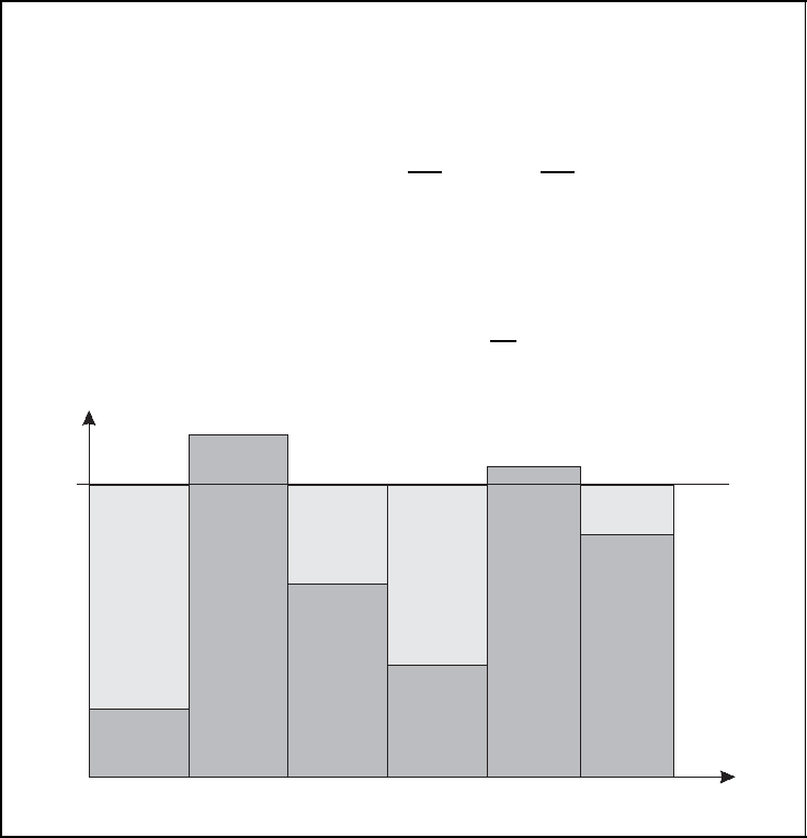
using Lagrangian multipliers, the famous waterﬁlling solution is obtained. It is illustrated in

Figure 5.25, where each bin represents one of the scalar channels. We have to imagine the

SPACE–TIME CODES 247

Waterﬁlling solution

■ Waterﬁlling solution

X ,i







θ −

H,i

for θ>

H,i

0 else

(5.51)

■ Total transmit power constraint



i=1

X ,i

= N

(5.52)

channel ν

/σ

H,1

/σ

H,2

/σ

H,3

/σ

H,4

/σ

H,5

/σ

H,6

X ,1

X ,2

= 0

X ,3

X ,4

X ,5

= 0

X ,6

Figure 5.25: Waterﬁlling solution. Reproduced by permission of John Wiley & Sons, Ltd

diagram as a vessel with a bumpy ground where the height of the ground is proportional

to the ratio σ

/σ

H,i

. Pouring water into the vessel is equivalent to distributing transmit

power onto the parallel scalar channels. The process is stopped when the totally available

transmit power is consumed. Obviously, good channels with a low σ

/σ

H,i

obtain more

transmit power than weak channels. The worst channels whose bins are not covered by

the water level θ do not obtain any power, which can also be seen from Equation (5.51).

Therefore, we can conclude that much power is spent on good channels transmitting high

data rates, while little power is given to bad channels transmitting only very low data rates.

This strategy leads to the highest possible data rate.

248 SPACE–TIME CODES

Channel capacity and receive diversity

0 5 10 15 20

in dB →

C →

= 1N

= 1

= 2N

= 2

= 3N

= 3

= 4N

= 4

in dB per receive antenna

(a) SNR per receive antenna

(b) SNR after combining

Figure 5.26: Channel capacity and receive diversity. Reproduced by permission of John

Wiley & Sons, Ltd

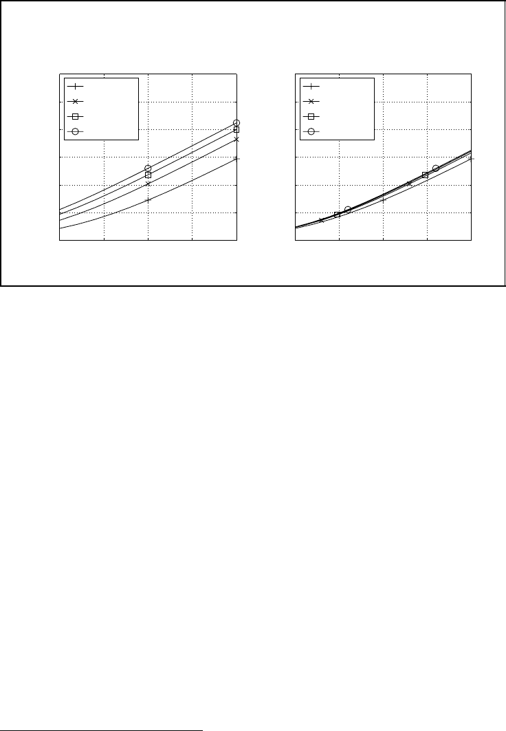
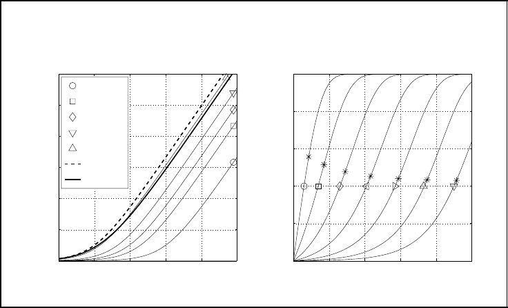
Figure 5.26 illuminates array and diversity gains for a system with a single transmit and

several receive antennas. In the left-hand diagram, the ergodic capacity is plotted versus

the signal-to-noise ratio at each receive antenna. The more receive antennas employed, the

more signal energy can be collected. Hence, doubling the number of receive antennas also

doubles the SNR after maximum ratio combining, resulting in a 3 dB gain. This gain is

denoted as array gain.

Additionally, a diversity gain can be observed, stemming from the

fact that variations in the SNR owing to fading are reduced by combining independent

diversity paths. Both effects lead to a gain of approximately 6.5 dB by increasing the

number of receive antennas from N

= 1toN

= 2. This gain reduces to 3.6 dB by going

from N

= 2toN

= 4. The array gain still amounts to 3 dB, but the diversity gain is

getting smaller if the number of diversity paths is already high.

The pure diversity gains become visible in the right-hand diagram plotting the ergodic

capacities versus the SNR after maximum ratio combining. This normalisation removes

the array gain, and only the diversity gain remains. We observe that the ergodic capacity

increases only marginally owing to a higher diversity degree.

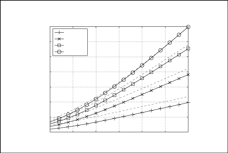
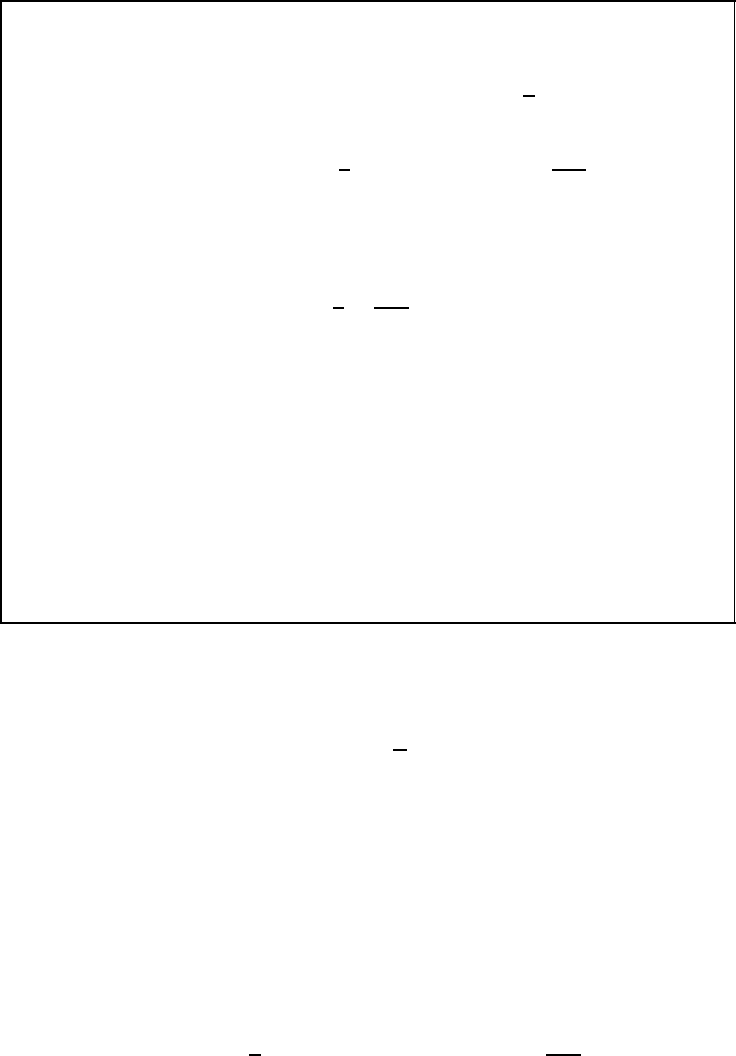
Figure 5.27 shows the ergodic capacities for a system with N

= 4 transmit antennas

versus the signal-to-noise ratio E

. The MIMO channel matrix consists of i.i.d. com-

plex circular Gaussian distributed coefﬁcients. Solid lines represent the results with perfect

channel knowledge only at the receiver, while dashed lines correspond to the waterﬁlling

solution with ideal CSI at transmitter and receiver. Asymptotically for large signal-to-noise

ratios, we observe that the capacities increase linearly with the SNR. The slope amounts

Certainly, the receiver cannot collect a higher signal power than has been transmitted. However, the channels’

path loss has been omitted here so that the average channel gains are normalised to unity.

SPACE–TIME CODES 249

Ergodic capacity of MIMO systems

0 5 10 15 20 25 30

in dB →

C →

= 1

= 2

= 3

= 4

Figure 5.27: Ergodic capacity of MIMO systems with N

= 4 transmit antennas and

varying N

(solid lines: CSI only at receiver; dashed lines: waterﬁlling solution with

perfect CSI at transmitter and receiver)

to 1 bit/s/Hz for N

= 1, 2 bit/s/Hz for N

= 2, 3 bit/s/Hz for N

= 3 and 4 bit/s/Hz for

= 4, and therefore depends on the rank r of H. For ﬁxed N

= 4, the number of non-

zero eigenmodes r grows with the number of receive antennas up to r

max

= rank(H) = 4.

These data rate enhancements are called multiplexing gains because we can transmit up to

max

parallel data streams over the MIMO channel. This conﬁrms our theoretical results

that the capacity increases linearly with the rank of H while it grows only logarithmically

with the SNR.

Moreover, we observe that perfect CSI at the transmitter leads to remarkable improve-

ments for N

. For these conﬁgurations, the rank of our system is limited by the

number of receive antennas. Exploiting the non-zero eigenmodes requires some kind of

beamforming which is only possible with appropriate channel knowledge at the transmit-

ter. For N

= 1, only one non-zero eigenmode exists. With transmitter CSI, we obtain

an array gain of 10 log

(4) ≈ 6 dB which is not achievable without channel knowledge.

For N

= N

= 4, the additional gain due to channel knowledge at the transmitter is vis-

ible only at low SNR where the waterﬁlling solution drops the weakest eigenmodes and

concentrates the transmit power only on the strongest modes, whereas this is impossible

without transmitter CSI. At high SNR, the water level in Figure 5.25 is so high that all

eigenmodes are active and a slightly different distribution of the transmit power has only

a minor impact on the ergodic capacity.

250 SPACE–TIME CODES

5.3.2 Outage Probability and Outage Capacity

As we have seen from Figure 5.22, the channel capacity of fading channels is a random

variable itself. The average capacity is called the ergodic capacity and makes sense if the

channel varies fast enough so that one coded frame experiences the full channel statistics.

Theoretically, this assumes inﬁnite long sequences due to the channel coding theorem. For

delay-limited applications with short sequences and slowly fading channels, the ergodic

capacity is often not meaningful because a coded frame is affected by an incomplete part

of the channel statistics. In these cases, the ‘short-term capacity’ may vary from frame to

frame, and network operators are interested in the probability that a system cannot support

a desired throughput R. This parameter is termed the outage probability P

out

and is deﬁned

in Equation (5.53) in Figure 5.28.

Equivalently, the outage capacity C

describes the capacity that cannot be achieved in

p percent of all fading states. For the case of a Rayleigh fading channel, outage probability

and capacity are also presented in Figure 5.28. The outage capacity C

out

is obtained by

resolving the equation for P

out

with respect to R = C

out

. For MIMO channels, we sim-

ply have to replace the expression of the scalar capacity with that for the multiple-input

multiple-output case.

Outage probability of fading channels

■ Outage probability of a scalar channel

out

= Pr{C[k] <R}=Pr{|h[k]|

− 1

} (5.53)

– Outage probability for scalar Rayleigh fading channels (K

uhn, 2006)

out

= 1 −exp



1 − 2



– Outage capacity for scalar Rayleigh fading channel

out

= log



1 − E

· log(1 −P

out

)



■ Outage probability for MIMO channel with singular values σ

H,i

out

= Pr{C[k] <R}=Pr{



µ=1

log

1 + σ

H,i

X ,i

<R} (5.54)

Figure 5.28: Outage probability of fading channels

SPACE–TIME CODES 251

Capacity and outage probability of Rayleigh fading channels

Ŧ10 0 10 20 30 40

0 2 4 6 8 10

0.2

0.4

0.6

0.8

in dB →

(a)

C →

AWGN

(b)

out

→

R →

0dB

5dB

10dB

15dB20dB

25dB30dB

Figure 5.29: Capacity and outage probability of Rayleigh fading channels

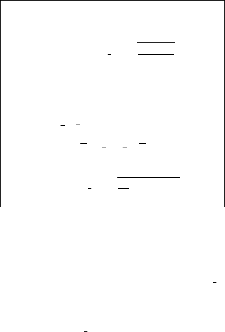
The left-hand diagram in Figure 5.29 shows a comparison between the ergodic capac-

ities of AWGN and ﬂat Rayleigh fading channels (bold lines). For sufﬁciently large SNR,

the curves are parallel and we can observe a loss due to fading of roughly 2.5 dB. Com-

pared with the loss of approximately 17 dB at a bit error rate (BER) of P

= 10

−3

in the uncoded case, the observed difference is rather small. This discrepancy can be

explained by the fact that the channel coding theorem presupposes inﬁnite long code words

allowing the decoder to exploit a high diversity gain. Therefore, the loss in capacity com-

pared with the AWGN channel is relatively small. Astonishingly, the ultimate limit of

10 log

) =−1.59 dB is the same for AWGN and Rayleigh fading channels.

Additionally, the left-hand diagram shows the outage capacities for different values of

out

. For example, the capacity C

can be ensured with a probability of 50% and is close

to the ergodic capacity

C. The outage capacities C

decrease dramatically for smaller P

out

i.e. the higher the requirements, the higher is the risk of an outage event. At a spectral

efﬁciency of 6 bit/s/Hz, the loss compared with the AWGN channel in terms of E

amounts to nearly 8 dB for P

out

= 0.1 and roughly 18 dB for P

out

= 0.01.

The right-hand diagram depicts the outage probability versus the target throughput R

for different values of E

. As expected for large signal-to-noise ratios, high data rates

can be guaranteed with very low outage probabilities. However, P

out

grows rapidly with

decreasing E

. The asterisks denote the outage probability of the ergodic capacity

R =

C. As could already be observed in the left-hand diagram, it is close to a probability

of 0.5.

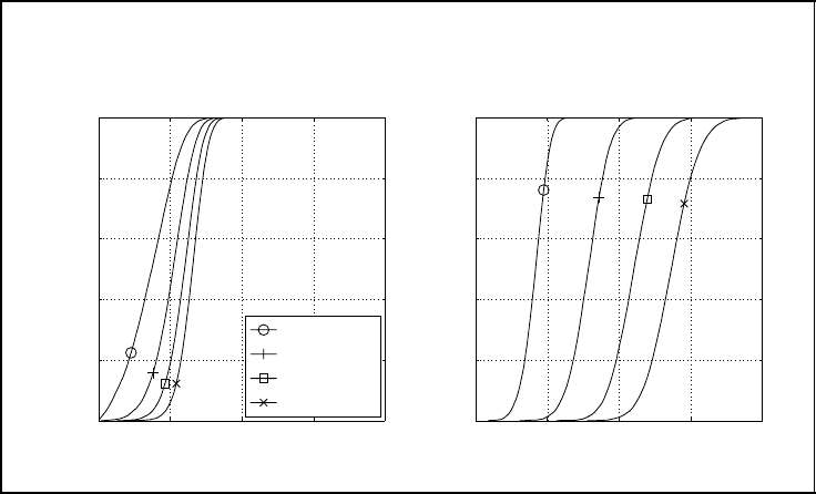
Finally, Figure 5.30 shows the outage probabilities for 1 × N

and 4 ×N

MIMO

systems at an average signal-to-noise ratio of 10 dB. From ﬁgure (a) it becomes obvious

252 SPACE–TIME CODES

Outage probability of MIMO fading channels

0 4 8 12 16

0.2

0.4

0.6

0.8

0 4 8 12 16

0.2

0.4

0.6

0.8

out

→

out

→

R →R →

(a) N

= 1

(b) N

= 4

= 1

= 2

= 3

= 4

Figure 5.30: Outage probability of MIMO fading channels

that an increasing number of receive antennas enlarges the diversity degree and, hence,

minimises the risk of an outage event. However, there is no multiplexing gain with only a

single transmit antenna, and the gains for additional receive antennas become smaller if the

number of receiving elements is already large. This is a well-known effect from diversity,

assuming an appropriate scaling of the signal-to-noise ratio. In ﬁgure (b), the system with

= 4 transmit antennas is considered. Here, we observe larger gains with each additional

receive antenna, since the number of eigenmodes increases so that we obtain a multiplexing

gain besides diversity enhancements.

5.3.3 Ergodic Error Probability

Having analysed MIMO systems on an information theory basis, we will now have a look at

the error probabilities. The following derivation was ﬁrst introduced for space–time codes

(Tarokh et al., 1998). However, it can be applied to general MIMO systems. It assumes

an optimal maximum likelihood detection and perfect channel knowledge at the receiver

and a block-wise transmission, i.e. L consecutive vectors x[k] are written into the N

× L

transmit matrix

X =

x[0] x[1] ···x[L − 1]







[0] x

[1] ··· x

[L − 1]

[0] x

[1] ··· x

[L − 1]

[0] x

[1] ··· x

[L − 1]







SPACE–TIME CODES 253

The MIMO channel is assumed to be constant during L time instants so that we receive

an N

× L matrix R

R =

r[0] r[1] ···r[L − 1]







[0] r

[1] ··· r

[L − 1]

[0] r

[1] ··· r

[L − 1]

[0] r

[1] ··· r

[L − 1]







= H · X + N ,

where N contains the noise vectors n[k] within the considered block. The set of all possible

matrices X is termed X. In the case of a space–time block code, certain constraints apply

to X, limiting the size of X (see Section 5.4). By contrast, for the well-known Bell Labs

Layered Space–Time (BLAST) transmission, there are no constraints on X, leading to a

size |X|=M

, where M is the size of the modulation alphabet.

Calculating the average error probability generally starts with the determination of the

pairwise error probability Pr{B →

B | H}. Equivalently to the explanation in Chapter 3, it

denotes the probability that the detector decides in favour of a code matrix

X although X

was transmitted. Assuming uncorrelated noise contributions at each receive antenna, the

optimum detector performs a maximum likelihood estimation, i.e. it determines that code

matrix

X which minimises the squared Frobenius distance R − H

X

(see Appendix B

on page 312). Hence, we have to consider not the difference X −

X

, but the difference

in the noiseless received signals HX − H

X

, as done in Equation (5.55) in Figure 5.31.

In order to make the squared Frobenius norm independent of the average power E

a symbol, we normalise the space–time code words by the average power per symbol to

B =

√

and

B =

√

If the µth row of H is denoted by h

, the squared Frobenius norm can be written as

H(B −

(B −



µ=1

(B −

B)(B −

This rewriting and the normalisation lead to the form given in Equation (5.56). We now

apply the eigenvalue decomposition on the Hermitian matrix

(B −

B)(B −

= UU

The matrix  is diagonal and contains the eigenvalues λ

of (B −

B)(B −

, while U is

unitary and consists of the corresponding eigenvectors. Inserting the eigenvalue decompo-

sition into Equation (5.56) yields

H(B −



µ=1

U ·  · U



µ=1

β

with β

= [β

µ,1

, ... , β

µ,L

]. Since  is diagonal, its multiplication with β

and β

from

the left- and the right-handside respectively reduces to

H(B −



µ=1



ν=1

|β

µ,ν

· λ



µ=1



ν=1

|β

µ,ν

· λ

254 SPACE–TIME CODES

Pairwise error probability

■ Pairwise error probability for code matrices X and

Pr{X →

X | H}=

· erfc







(

)

HX − H

4σ







(5.55)

■ Normalisation to unit average power per symbol

H · (X −



µ=1

· (B −

B)(B −

· h

(5.56)

■ Substitution of β

= h

H · (X −



µ=1

·  · β



µ=1



ν=1

|β

· λ

(5.57)

■ With σ

= N

, pairwise error probability becomes

Pr{X →

X | H}=

· erfc





(

)



µ=1



ν=1

|β

µ,ν

· λ





(5.58)

Figure 5.31: Pairwise error probability for space–time code words

Assuming that the rank of  equals rank{}=r ≤ L, i.e. r eigenvalues λ

are non-zero,

the inner sum can be restricted to run from ν = 1 only to ν = r because λ

ν>r

= 0 holds.

The last equality is obtained because  is diagonal. Inserting the new expression for the

squared Frobenius norm into the pairwise error probability of Equation (5.55) delivers the

result in Equation (5.58).

The last step in our derivation starts with the application of the upper bound erfc(

√

x) <

−x

on the complementary error function. Rewriting the double sum in the exponent into the

product of exponential functions leads to the result in inequality (5.59) in Figure 5.32. In

order to obtain a pairwise error probability averaged over all possible channel observations,

the expectation of Equation (5.58) with respect to H has to be determined. This expectation

is calculated over all channel coefﬁcients h

µ,ν

of H. At this point it has to be mentioned

that the multiplication of a vector h

with U performs just a rotation in the N

-dimensional

SPACE–TIME CODES 255

Determinant and rank criteria

■ Upper bound on pairwise error probability by erfc(

√

x) < e

−x

Pr{B →

B | H}≤



µ=1



ν=1

exp

−|β

(5.59)

■ Expectation with respect to H yields

Pr{B →

B}≤





ν=1



1/r

−rN

(5.60)

■ Rank criterion: maximise the minimum rank of



B −



= N

· min

(B,

rank



B −



(5.61)

■ Determinant criterion: maximise the minimum of (

ν=1

)

1/r

= min

(B,





ν=1



1/r

(5.62)

Figure 5.32: Determinant and rank criteria

space. Hence the coefﬁcients β

µ,ν

of the vector β

have the same statistics as the channel

coefﬁcients h

µ,ν

(Naguib et al., 1997).

Assuming the frequently used case of independent Rayleigh fading, the coefﬁcients

µ,ν

, and, consequently also β

µ,ν

, are complex rotationally invariant Gaussian distributed

random variables with unit power σ

= 1. Hence, their squared magnitudes are chi-squared

distributed with two degrees of freedom, i.e.

µ,ν

(ξ) = e

−ξ

holds. The expectation of inequality (5.59) now results in

Pr{B →

B}=E



Pr{B →

B | H}

≤



µ=1



ν=1

exp

− λ

·|β

µ,ν