Omran M.G.H. Particle Swarm Optimization Methods for Pattern Recognition and Image Processing

Подождите немного. Документ загружается.

150

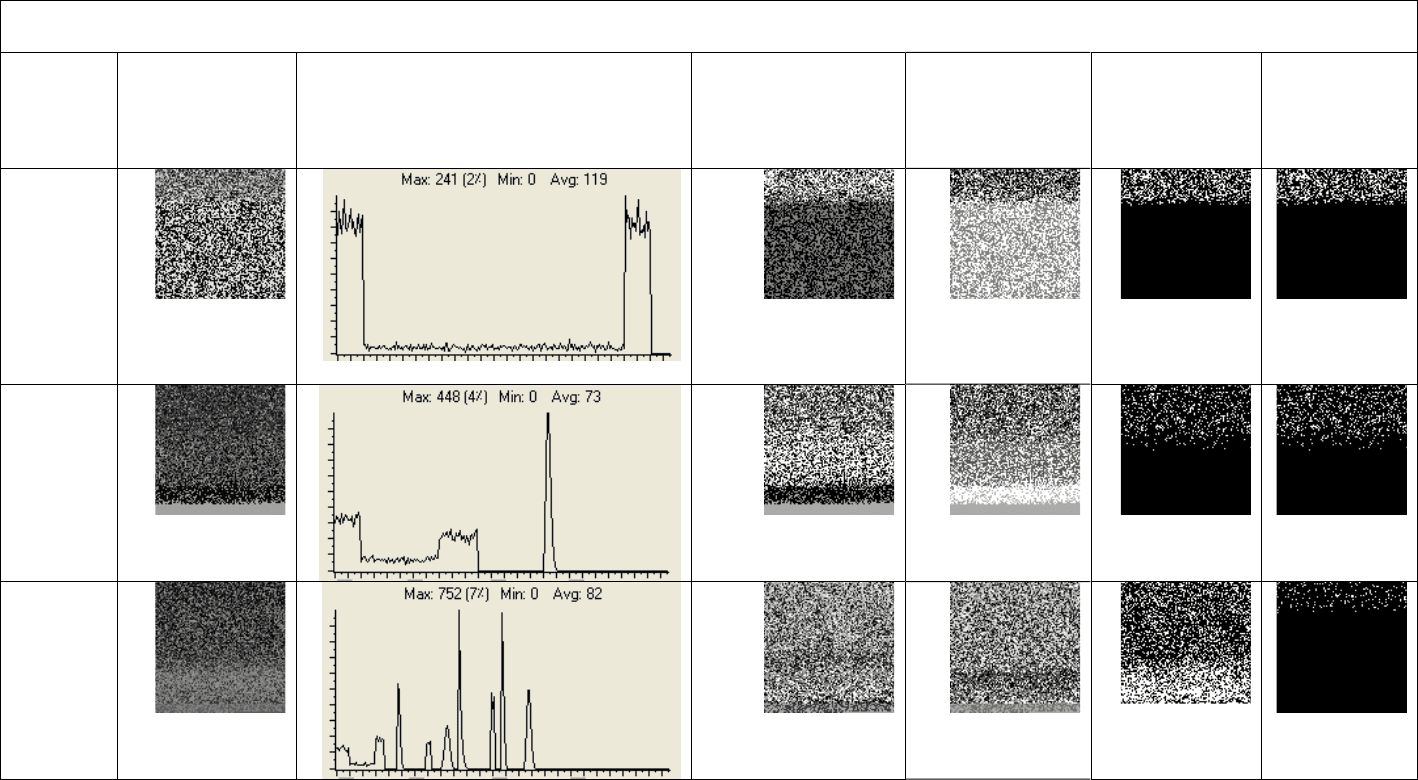
Table 5.2 (continued).

Bench

Mark No.

Synthetic Image Histogram

K-Means Sample TM

(Avg. Classification

Accuracy

±SD)

[CI]

PSO Sample TM

(Avg. Classification

Accuracy

±SD)

[CI]

Best K-Means

TM Difference

(Best

Classification

Accuracy)

Best PSO TM

Difference

(Best

Classification

Accuracy)

90.56%±0

[90.560, 90.560]

90.69%±0.060

[90.664, 90.707]

(90.56%)

(90.77%)

91.75%±7.647

[89.018, 94.490]

92.18%±0.318

[92.070, 92.298]

(93.21%)

(92.48%)

50.91%±9.543

[47.494, 54.323]

60.53%±26.043

[51.213, 69.852]

(56.71%)

(98.11%)

151

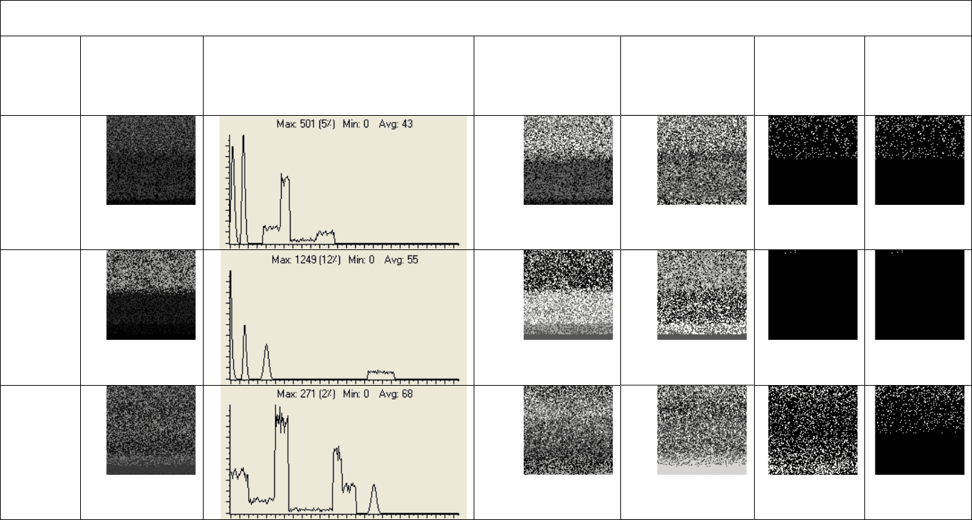
Table 5.2 (continued).

Bench

Mark No.

Synthetic Image Histogram

K-Means Sample TM

(Avg. Classification

Accuracy

±SD)

[CI]

PSO Sample TM

(Avg. Classification

Accuracy

±SD)

[CI]

Best K-Means

TM Difference

(Best

Classification

Accuracy)

Best PSO TM

Difference

(Best

Classification

Accuracy)

60.62%±27.284

[50.856, 70.383]

77.14%±14.021

[72.119, 82.154]

(95.81%)

(95.59%)

99.96%±0

[99.96, 99.96]

99.96%±0

[99.96, 99.96]

(99.96%)

55.23%±20.975

[47.723, 62.734]

60.19%±13.428

[55.384, 64.995]

(75.99%)

(94.08%)

152

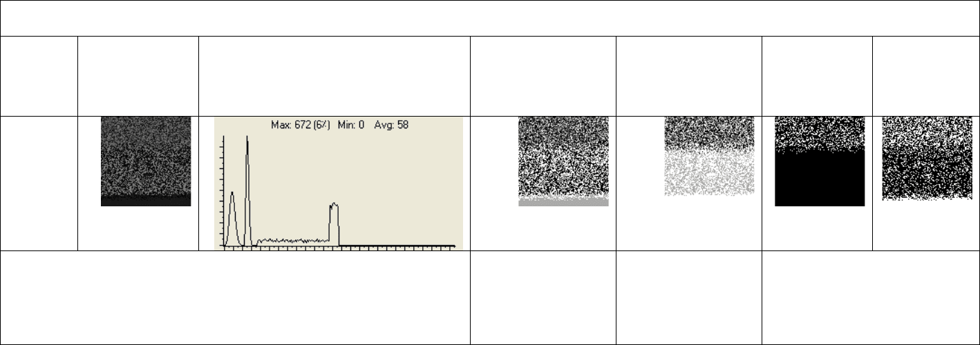
Table 5.2 (continued).

Bench

Mark

No.

Synthetic

Image

Histogram

K-Means Sample TM

(Avg. Classification

Accuracy

±SD)

[CI]

PSO Sample TM

(Avg. Classification

Accuracy

±SD)

[CI]

Best K-Means

TM Difference

(Best

Classification

Accuracy)

Best PSO TM

Difference

(Best

Classification

Accuracy)

88.83%±0

[88.83, 88.83]

60.14%±0.211

[60.065, 60.216]

(88.83%)

(60.47%)

Average Performance

81.74%±18.25123

[70.43,93.05]

83.73%±16.63667

[73.41,94.04]

153

Chapter 6

Dynamic Clustering using Particle Swarm

Optimization with Application to Unsupervised Image

Classification

A new dynamic clustering approach (DCPSO), based on PSO, is proposed in this chapter.

This approach is applied to unsupervised image classification. The proposed approach

automatically determines the "optimum" number of clusters and simultaneously clusters the

data set with minimal user interference. The algorithm starts by partitioning the data set into a

relatively large number of clusters to reduce the effects of initial conditions. Using binary

particle swarm optimization the "best" number of clusters is selected. The centroids of the

chosen clusters are then refined via the K-means clustering algorithm. The proposed approach

is then applied on synthetic, natural and multispectral images. The experiments conducted

show that the proposed approach generally found the "optimum" number of clusters on the

tested images. A genetic algorithm and a random search version of dynamic clustering are

presented and compared to the particle swarm version.

6.1 The Dynamic Clustering using PSO (DCPSO) Algorithm

This section presents the DCPSO algorithm. For this purpose, define the following

symbols:

is the maximum number of clusters.

is the dimension of the data set.

154

is the number of patterns to be clustered.

Z = {z

j,p

∈ ℜ | j = 1,…, N

and p = 1,…, N

} is the set of patterns.

M = {m

j,k

∈

ℜ

| j = 1,…, N

and k = 1,…, N

} is the set of N

cluster centroids.

= {x

,…, x

} is the swarm of s particles such that x

indicates particle i, with

i,k

∈ {0,1} for k = 1,…, N

such that if x

i,k

= 1 then the corresponding centroid m

M has been chosen to be part of the solution proposed by particle x

. Otherwise, if x

i,k

= 0 then the corresponding

in M is not part of the solution proposed by x

is the number of clusters used by the clustering solution represented by particle x

such that

∑

ji,i

, with n

≤ N

is the clustering solution represented by particle x

such that M

= (m

) ∀ k: x

i,k

= 1

with

⊆ M.

n is the number of clusters used by the clustering solution represented by the global

best particle

(assuming that gbest PSO is used) such that

∑

kτ

, with

n ≤ N

is the clustering solution represented by y

such that M

= (m

) ∀ k:

= 1 with

⊆ M.

is the set of centroids in M which have not been chosen by

, i.e. M

= (m

), ∀ k:

= 0 with M

⊆ M (i.e. M

∩ M

= ∅ and M

∪ M

= M).

ini

is a user-specified probability defined in Kuncheva and Bezdek [1998], which is

used to initialize a particle position,

, as follows:

155







≥

ini

)( if 1

)( if 0

)(

ptr

ki,

(6.1)

where (0,1))( U~tr

. Obviously a large value for p

ini

results in selecting most of the

centroids in

The algorithm which uses some of the ideas presented by Kuncheva and Bezdek

[1998]: A pool of cluster centroids,

M, is randomly chosen from Z. The swarm of

particles,

S, is then randomly initialized. Binary PSO is then applied to find the "best"

set of cluster centroids,

, from M. K-means is applied to M

in order to refine the

chosen centroids.

M is then set to M

plus M

which is a randomly chosen set of

centroids from

Z (this is done to add diversity to M and to reduce the effect of the

initial conditions). The algorithm is then repeated using the new

M. When the

termination criteria are met,

will be the resulting "optimum" set of cluster

centroids and

n will be the "optimum" number of clusters in Z. The DCPSO

algorithm is summarized in Figure 6.1.

The termination criterion can be a user-defined maximum number of iterations

or a lack of progress in improving the best solution found so far for a user-specified

consecutive number of iterations, TC. In this chapter, the latter approach is used with

= 50 for Step 6 and TC

= 2 for step 10. These values for TC were set empirically.

and s are user defined parameters.

156

Select m

∈ M, ∀ k = 1,…, N

where 1 < N

< N

, randomly from Z

Initialize the swarm S, with x

i,k

~ U{0,1}, ∀ i = 1,…, s and k = 1,…, N

using

equation (6.1)

Randomly initialize the velocity, v

, of each particle i in S such that

5,5][−∈

ki,

v , ∀ i = 1,…, s and k = 1,…, N

. The range of [-5,5] was set

empirically

For each particle x

in S

Partition Z according to the centroids in M

by assigning each data

point

to the closest (in terms of the Euclidean distance) cluster in M

Calculate the clustering validity index, VI, using one of the clustering

validity indices as defined in section 3.1.4 to measure the quality of the

resulting partitioning of

Z (i.e. VI = V, VI = S_Dbw or VI=1/D since D

should be maximized)

f(x

) = VI

Apply the binary PSO velocity and position update equations (2.8) and (2.15)

on all particles in

Repeat steps 4) and 5) until a termination criterion is met

Adjust M

by applying the K-means clustering algorithm

Randomly re-initialize M

from Z

Set M = M

∪ M

10)

Repeat steps 2) through 9) until a termination criterion is met

Figure 6.1: The DCPSO algorithm

157

A GA version of DCPSO can easily be implemented by replacing step 5 in the above

algorithm with GA evolutionary operators for selection, crossover and mutation. On

the other hand, a random search (RS) version of DCPSO, as described by Kunchevea

and Bezdek [1998], can be implemented by removing step 5 and keeping only the best

solution encountered so far.

As an illustration of the DCPSO algorithm, consider the following example.

Example 6.1

Let N

= 100, N

= 1, and N

= 5.

Let

M be

3 29 78 150 200

An example of a particle position,

, is

0 1 1 0 1

which means that cluster centers 29, 78 and 200 are chosen for this particle such that

29 78 200

In other words, all data in

Z are grouped in only these three clusters.

After step 6, assume the global best particle,

, is

0 1 0 1 1

Then,

158

29 150 200

Assume that after K-means is applied on

Z using the centroids given by M

, the new

is given by

30.5 129.9 201

Then, randomly initialize the remaining N

- n

(i.e. 5 - 3 = 2) clusters, representing

, from Z (shown below in bold). The resultant M may look as follows:

110

30.5

129.9 201

The DCPSO algorithm is then repeated using the new

6.1.1 Validity Index

One of the advantages of DCPSO is that it can use any validity index. Therefore, the

user can choose the validity index suitable for his/her data set. In addition, any new

index can easily be integrated with DCPSO. The validity indices used in this chapter

are D, V and S_Dbw (as defined in section 3.1.4).

6.1.2 Time Complexity

The time complexity of DCPSO is based on the complexity of four processes, namely,

the partitioning of

Z, calculating the quality of the partition, applying binary PSO and

applying K-means. Assume that T

is the number of iterations taken by the PSO to

159

converge (step 6 of the algorithm), and that T

is the number of iterations taken by

DCPSO to converge (step 10 of the algorithm). Then the complexity of partitioning

is O(sT

), while the complexity of calculating the quality of a partition will

depend on the time complexity of the validity index which is, in general, some

constant, ξ, multiplied by N

for the indices used in this chapter. The complexity of

this step is therefore O(ξT

). Finally, the complexity of K-means is O(N

). The

parameters T

, T

, s and ξ can be fixed in advance. Typically, T

, T

, s, ξ, N

. Let ς be the multiplication of s, T

, T

, N

and N

(i.e. ς = sT

). If

N<<ς

then the time complexity of DCPSO will be

O(N

). However, if

≈

ς then the time

complexity of DCPSO will be O(

6.2 Experimental results

Experiments were conducted using both synthetic images and natural images. The

synthetic images were generated by SIGT as given in Table 5.1. Furthermore, SIGT

was used to generate another five different synthetic images for which the actual

number of clusters was known in advance. These images have different numbers of

clusters with varying complexities; they consist of well separated clusters,

overlapping clusters or a combination of both. The new five synthetic images are

given in Table 6.1 along with their histograms.

The following well known natural images were used:

Lenna, mandrill, jet and

peppers. These images are shown in Figure 6.2. Furthermore, one MRI and one

satellite image of Lake Tahoe (as given in Figure 4.2) have been used to show the

wide applicability of the proposed approach.