Patrick F. Dunn, Measurement, Data Analysis, and Sensor Fundamentals for Engineering and Science, 2nd Edition
Подождите немного. Документ загружается.


196 Measurement and Data Analysis for Engineering and Science
ν t
ν,P =50 %
t
ν,P =90 %
t
ν,P =95 %
t
ν,P =99 %
1 1.000 6.341 12.706 63.657
2 0.816 2.920 4.303 9.925
3 0.765 2.353 3.192 5.841
4 0.741 2.132 2.770 4.604
5 0.727 2.015 2.571 4.032
6 0.718 1.943 2.447 3.707
7 0.711 1.895 2.365 3.499
8 0.706 1.860 2.306 3.355
9 0.703 1.833 2.262 3.250
10 0.700 1.812 2.228 3.169
11 0.697 1.796 2.201 3.106
12 0.695 1.782 2.179 3.055
13 0.694 1.771 2.160 3.012
14 0.692 1.761 2.145 2.977
15 0.691 1.753 2.131 2.947
16 0.690 1.746 2.120 2.921
17 0.689 1.740 2.110 2.898
18 0.688 1.734 2.101 2.878
19 0.688 1.729 2.093 2.861
20 0.687 1.725 2.086 2.845
21 0.686 1.721 2.080 2.831
30 0.683 1.697 2.042 2.750
40 0.681 1.684 2.021 2.704
50 0.680 1.679 2.010 2.679
60 0.679 1.671 2.000 2.660
120 0.677 1.658 1.980 2.617
∞ 0.674 1.645 1.960 2.576
TABLE 6.4
Student’s t variable values for different P and ν.
Statistics 197
99.73 %
95.45 %
68.27 %
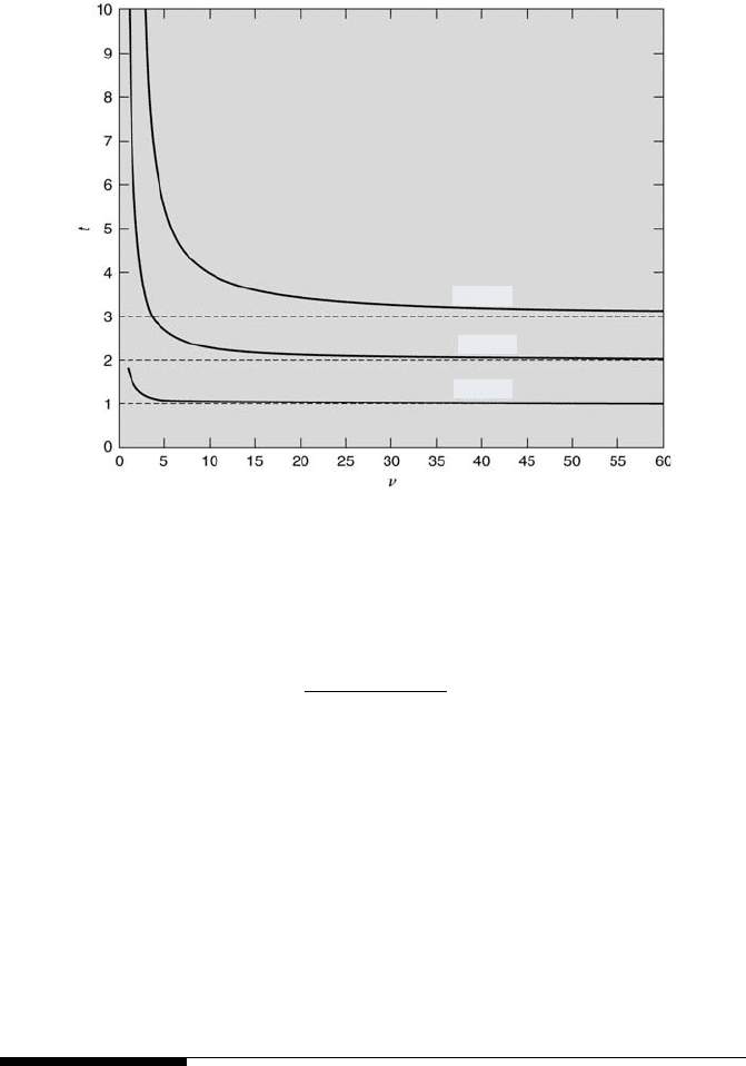
FIGURE 6.5
Student’s t values for various degrees of freedom and percent probabilities.
This is
t
ν,P
= ±
(x
0
− ¯x) ± z
P
σ
S
x
(% P ). (6.24)
Now, in the limit as N → ∞, the sample mean, ¯x, tends to the true mean, x
0
,
and the sample standard deviation, S
x
, tends to the true standard deviation
σ. It follows from Equation 6.24 that t
ν,P
tends to z
P
. This is illustrated in
Figure 6.5, in which the t
ν,P
values for P = 68.27 %, 95.45 % and 99.73 %
are plotted versus ν. This figure was constructed using the MATLAB M-file
tnuP.m. As shown in the figure, for increasing values of ν, the t
ν,P
values for
P = 68.27 %, 95.45 % and 99.73 % approach the z
P
values of 1, 2, and 3,
respectively. In other words, Student’s t distribution approaches the normal
distribution as N tends to infinity.
6.5 Standard Deviation of the Means
Consider a sample of N measurands. From its sample mean, ¯x, and its
sample standard deviation, S
x
, the region within which the true mean of
the underlying population, x
0
, can be inferred. This is done by statistically
198 Measurement and Data Analysis for Engineering and Science
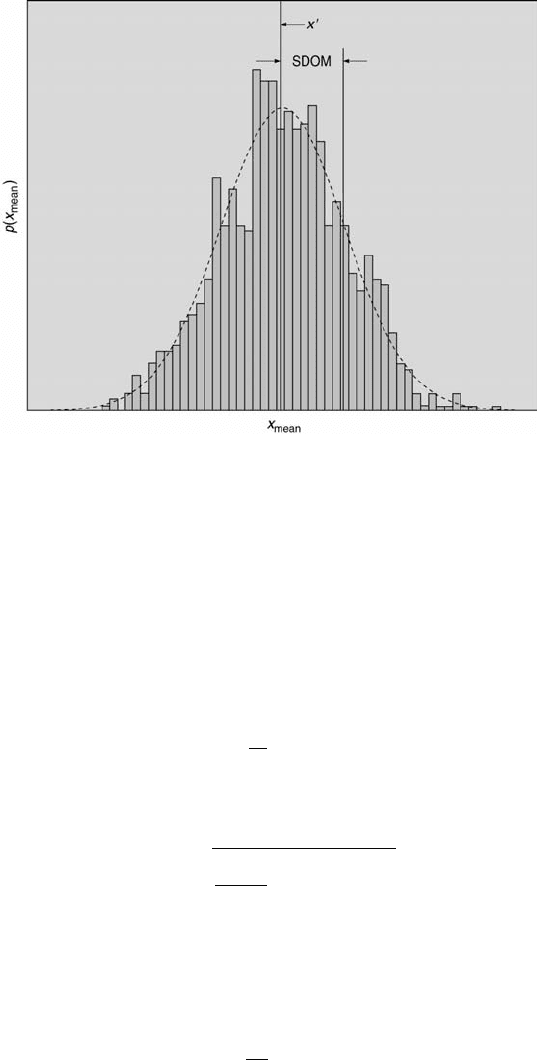
FIGURE 6.6
The probability density function of the mean values of x.
relating the sample to the population through the standard deviation of
the means (SDOM).
Assume that there are M sets (samples), each comprised of N measur-
ands. A specific measurand value is denoted by x
ij
, where i = 1 to N refers
to the specific number within a set and j = 1 to M refers to the particular
set. Each set will have a mean value, ¯x
j
, where
¯x
j
=
1
N
N
X
i=1
x
ij
, (6.25)
and a sample standard deviation, S
x
j
, where
S
x
j
=
v
u
u
t
1
N − 1
N
X
i=1
(x
ij
− ¯x
j
)
2
. (6.26)
Now each ¯x
j
is a random variable. The central limit theorem assures
that the ¯x
j
values will be normally distributed about their mean value (the
mean of the mean values),
¯
¯x, where
¯
¯x =
1
M
M
X
j=1
¯x
j
. (6.27)

Statistics 199
This is illustrated in Figure 6.6.
The standard deviation of the mean values (termed the standard devia-
tion of the means), then will be
S
¯x
=
1
M − 1
M
X
j=1
(¯x −
¯
¯x)
2
1/2
. (6.28)
It can be proven using Equations 6.26 and 6.28 [4] that
S
¯x
= S
x
/
√
N. (6.29)
This deceptively simple formula allows us to determine from the values of
only one finite set the range of values that contains the true mean value of
the entire population. Formally
x
0
= ¯x ± t
ν,P
S
¯x
= ¯x ± t
ν,P
S
x
√
N
(% P ). (6.30)
This formula implies that the bounds within which x
0
is contained can be
reduced, which means that the estimate of x
0
can be made more precise, by
increasing N or by decreasing the value of S
x
. There is a moral here. It is
better to carefully plan an experiment to minimize the number of random
effects beforehand and hence to reduce S
x
, rather than to spend the time
acquiring more data to achieve the same bounds on x
0
.
The interval ±t
ν,P
S
¯x
is called the precision interval of the true
mean. As N becomes large, from Equation 6.29 it follows that the SDOM
becomes small and the sample mean value tends toward the true mean value.
In this light, the precision interval of the true mean value can be viewed as
a measure of the uncertainty in determining x
0
.
Example Problem 6.4
Statement: Consider the differential pressure transducer measurements in the pre-
vious example. What is the range within which the true mean value of the differential
pressure, p
0
, is contained?
Solution: Equation 6.30 reveals that
p
0
= ¯p ± t
ν,P
S
¯p
= ¯p ± t
ν,P
S
p
√
N
(% P )
= 4.97 ±
(2.101)(0.046)
√
19
= 4.97 ± 0.02 (95 %)
.
Thus, the true mean value is estimated at 95 % confidence to be within the range from
4.95 kPa to 4.99 kPa.
Finally, it is very important to note that although Equations 6.23 and
6.30 appear to be similar, they are uniquely different. Equation 6.23 is used
to estimate the range within which another x
i
value will be with a given

200 Measurement and Data Analysis for Engineering and Science
confidence, whereas Equation 6.30 is used to estimate the range that con-
tains the true mean value for a given confidence. Both equations use the
values of the sample mean, standard deviation, and number of measurands
in making these estimates.
6.6 Chi-Square Distribution
The range that contains the true mean of a population can be estimated
using the values from only a single sample of N measurands and Equa-
tion 6.30. Likewise, there is an analogous way of estimating the range that
contains the true variance of a population using the values from only one
sample of N measurands. The estimate involves using one more probability
distribution, the chi-square distribution.
The chi-square distribution is used in many statistical calculations. For
example, it can be used to determine the precision interval of the true vari-
ance, to quantify how well a sample matches an assumed parent distribution,
and to compare two samples of same or different size with one another. The
statistical variable, χ
2
, represents the sum of the squares of the differences
between the measured and expected values normalized by their variance.
Thus, the value of χ
2
is dependent upon the number of measurements, N,
at which the comparison is made, and, hence, the number of degrees of free-
dom, ν = N − 1. From this definition it follows that χ
2
is related to the
standardized variable, z
i
= (x
i
− x
0
)/σ, and the number of measurements
by
χ
2
=
N
X
i=1
z
2
i
=
N
X
i=1
(x
i
− x
0
)
2
σ
2
. (6.31)
χ
2
can be viewed as a quantitative measure of the total deviation of all
x
i
values from their population’s true mean value with respect to their
population’s standard deviation. This concept can be used, for example, to
compare the χ
2
value of a sample with the value that would be expected for
a sample of the same size drawn from a normally distributed population.
Using the definition of the sample variance given in Equation 6.21, this
expression becomes
χ
2
= νS
2
x
/σ
2
. (6.32)
So, in the limit as N → ∞, χ
2
→ ν.
The probability density function of χ
2
(for χ
2
≥ 0) is
p(χ
2
, ν) = [2
ν/2
Γ(ν/2)]
−1
(χ
2
)
(ν/2)−1
exp(−χ
2
/2), (6.33)
where Γ denotes the gamma function given by
Statistics 201
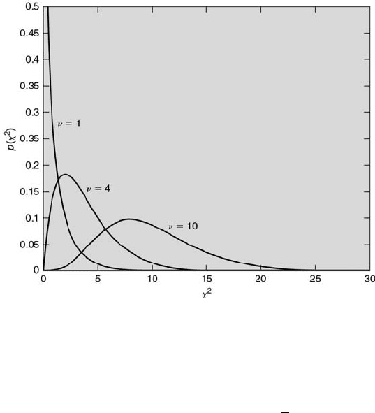
FIGURE 6.7
Three χ
2
probability density functions.
Γ(ν/2) =
Z
∞
0
x
(ν/2)−1
exp(−x)dx = (
ν
2
− 1)! (6.34)
and the mean and the variance of p(χ
2
, ν) are ν and 2ν, respectively. Some-
times values of χ
2
are normalized by the expected value, ν. The appropriate
parameter then becomes the reduced chi-square variable, which is de-
fined as
˜
χ
2
≡ χ
2
/ν. The mean value of the reduced chi-square variable
then equals unity. Finally, note that there is a different probability density
function of χ
2
for each value of ν.
The χ
2
probability density functions for three different values of ν are
plotted versus χ
2
in Figure 6.7. The MATLAB M-file chipdf.m was used
to construct this figure. The value of p(χ
2
= 10, ν = 10) is 0.0877, whereas
the value of p(χ
2
= 1, ν = 1) is 0.2420. For a sample of only N = 2
(ν = N − 1 = 1), there is almost a 100 % chance that the value of χ
2
will
be less than approximately 9. However, if N = 11 there is approximately a
50 % chance that the value of χ
2
will be less than approximately 9.
The corresponding probability distribution function, given by the inte-
gral of the probability density function from 0 to a specific value of χ
2
,
denoted by χ
2
α
, is called the chi-square distribution with ν degrees of free-
dom. It denotes the probability P (χ
2
α
) = 1 − α that χ
2
≤ χ
2
α
, where α
denotes the level of significance. In other words, the area under a spe-
cific χ
2
probability density function curve from 0 to χ
2
α
equals P (χ
2
α
) and
202 Measurement and Data Analysis for Engineering and Science
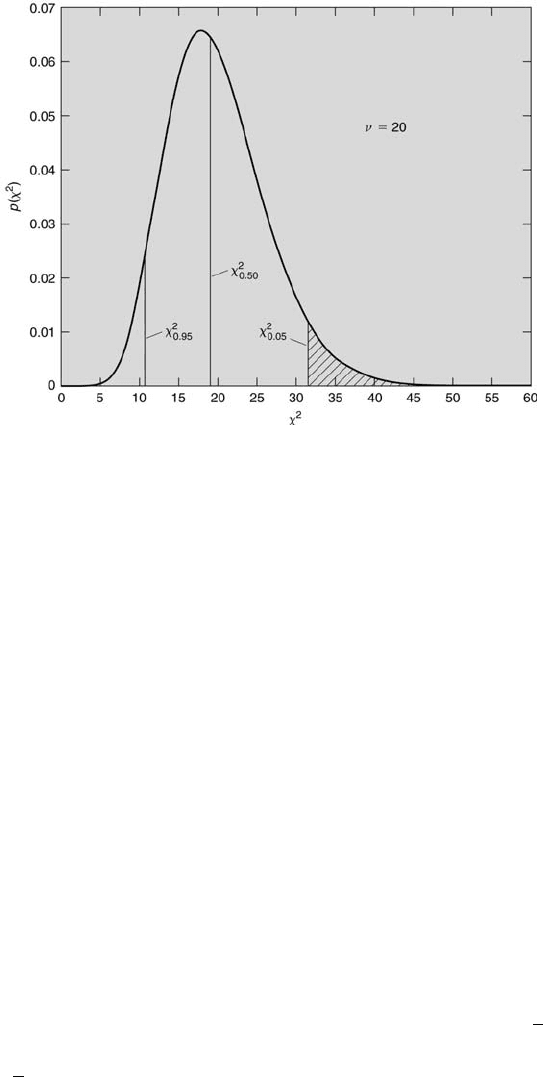
FIGURE 6.8
The χ
2
probability density function for ν = 20.
the area from χ
2
α
to ∞ equals α. The χ
2
probability density function for
ν = 20 is plotted in Figure 6.8. The MATLAB M-file chicdf.m was used
to construct this figure. Three χ
2
α
values (for α = 0.05, 0.50, and 0.95) are
indicated by vertical lines. The lined area represents 5 % of the total area
under the probability density curve, corresponding to α = 0.05. The χ
2
α
values for various ν and α are presented in Table 6.5. Using this table, for
ν = 20, χ
2
0.95
= 10.9, χ
2
0.50
= 19.3, and χ
2
0.05
= 31.4. That is, when ν = 20,
50 % of the area beneath the curve is between χ
2
= 0 and χ
2
= 19.3.
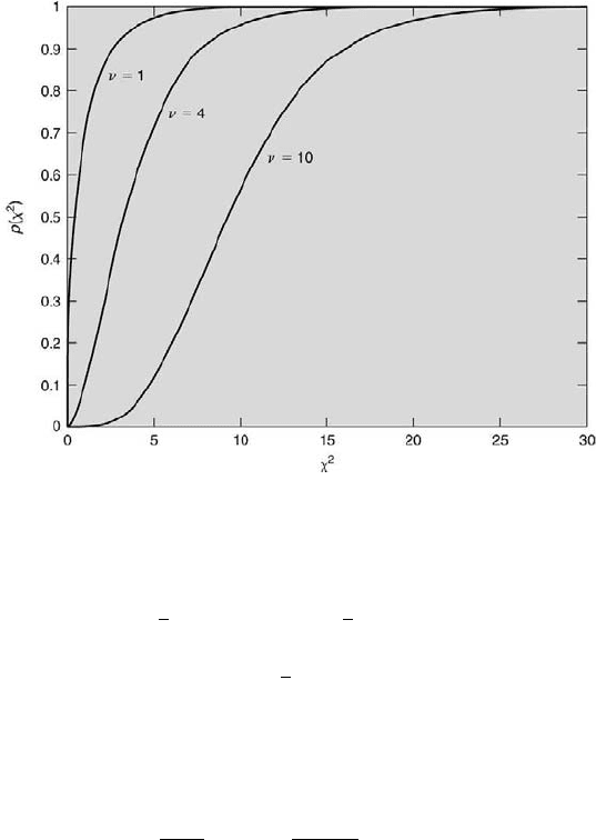
The χ
2
probability distribution functions for the same values of ν used
in Figure 6.7 are plotted versus χ
2
in Figure 6.9. For N = 2, there is a
99.73 % chance that the value of χ
2
will be less than 9. For N = 11, there
is a 46.79 % chance that the value of χ
2
will be less than 9. Finally, for
ν = 4, as already determined using Table 6.5, a value of χ
2
= 3.36 yields
P (χ
2
α
) = 0.50.
6.6.1 Estimating the True Variance
Consider a finite set of x
i
values drawn randomly from a normal distribution
having a true mean value x
0
and a true variance σ
2
. It follows directly from
Equation 6.32 and the definition of χ
2
α
that there is a probability of 1−
α
2
that
νS
2
x
/σ
2
≤ χ
2
α/2
or that νS
2
x
/χ
2
α/2
≤ σ
2
. Conversely, there is a probability of
1 − (1 −
α
2
) = α/2 that σ
2
≤ νS
2
x
/χ
2
α/2
. Likewise, there is a probability of

Statistics 203
ν χ
2
0.99
χ
2
0.975
χ
2
0.95
χ
2
0.90
χ
2
0.50
χ
2
0.05
χ
2
0.025
χ
2
0.01
1 0.000 0.000 0.000 0.016 0.455 3.84 5.02 6.63
2 0.020 0.051 0.103 0.211 1.39 5.99 7.38 9.21
3 0.115 0.216 0.352 0.584 2.37 7.81 9.35 11.3
4 0.297 0.484 0.711 1.06 3.36 9.49 11.1 13.3
5 0.554 0.831 1.15 1.61 4.35 11.1 12.8 15.1
6 0.872 1.24 1.64 2.20 5.35 12.6 14.4 16.8
7 1.24 1.69 2.17 2.83 6.35 14.1 16.0 18.5
8 1.65 2.18 2.73 3.49 7.34 15.5 17.5 20.1
9 2.09 2.70 3.33 4.17 8.34 16.9 19.0 21.7
10 2.56 3.25 3.94 4.78 9.34 18.3 20.5 23.2
11 3.05 3.82 4.57 5.58 10.3 19.7 21.9 24.7
12 3.57 4.40 5.23 6.30 11.3 21.0 23.3 26.2
13 4.11 5.01 5.89 7.04 12.3 22.4 24.7 27.7
14 4.66 5.63 6.57 7.79 13.3 23.7 26.1 29.1
15 5.23 6.26 7.26 8.55 14.3 25.0 27.5 30.6
16 5.81 6.91 7.96 9.31 15.3 26.3 28.8 32.0
17 6.41 7.56 8.67 10.1 16.3 27.6 30.2 33.4
18 7.01 8.23 9.39 10.9 17.3 28.9 31.5 34.8
19 7.63 8.91 10.1 11.7 18.3 30.1 32.9 36.2
20 8.26 9.59 10.9 12.4 19.3 31.4 34.2 37.6
30 15.0 16.8 18.5 20.6 29.3 43.8 47.0 50.9
40 22.2 24.4 26.5 29.1 39.3 55.8 59.3 63.7
50 29.7 32.4 34.8 37.7 49.3 67.5 71.4 76.2
60 37.5 40.5 43.2 46.5 59.3 79.1 83.3 88.4
70 45.4 48.8 51.7 55.3 69.3 90.5 95.0 100.4
80 53.5 57.2 60.4 64.3 79.3 101.9 106.6 112.3
90 61.8 65.6 69.1 73.3 89.3 113.1 118.1 124.1
100 70.1 74.2 77.9 82.4 99.3 124.3 129.6 135.8
TABLE 6.5
χ
2
α
values for various ν and α.
204 Measurement and Data Analysis for Engineering and Science
FIGURE 6.9
Three χ
2
probability distribution functions.
α/2 that νS
2
x
/σ
2
≤ χ
2
1−
α
2
or that νS
2
x
/χ
2
1−
α
2
≤ σ
2
. Thus, the true variance
of the underlying population, σ
2
, is within the sample variance precision
interval, from νS
2
x
/χ
2
α/2
to νS
2
x
/χ
2
1−
α
2
with a probability 1−(α/2)−(α/2) =
P . Also there is a probability α/2 that it is below the lower bound of the
precision interval, a probability α/2 that it is above the upper bound of the
precision interval, and a probability α that it is outside of the bounds of the
precision interval. Formally, this is
νS
2
x
χ
2
α/2
≤ σ
2
≤
νS
2
x
χ
2
1−α/2
(% P ). (6.35)
The width of the precision interval of the true variance in relation to
the probability P can be examined further. First consider the two extreme
cases. If P = 1 (100 %), then α = 0 which implies that χ
2
0
= ∞ and χ
2
1
= 0.
Thus, the sample variance precision interval is from 0 to ∞ according to
Equation 6.35. That is, there is a 100 % chance that σ
2
will have a value
between 0 and ∞. If P = 0 (0 %), then α = 1 which implies that the sample
variance precision intervals are the same. That is, there is a 0 % chance the
σ
2
will exactly equal one specific value out of an infinite number of possible
values (when α = 1 and ν >> 1, that unique value would be S
2
x
). These two
extreme-case examples illustrate the upper and lower limits of the sample
variance precision interval and its relation to P and α. As α varies from 0 to
1 (hence, P varies from 1 to 0), the precision interval width decreases from

Statistics 205
∞ to 0. In other words, the probability, α, that the true variance is outside
of the sample variance precision interval increases as the precision interval
width decreases.
6.6.2 Establishing a Rejection Criterion
The relation between the probability of occurrence of a χ
2
value being less
than a specified χ
2
value can be utilized to ascertain whether or not effects
other than random ones are present in an experiment or process. This is
particularly relevant, for example, in establishing a rejection criterion for a
manufacturing process or in an experiment. If the sample’s χ
2
value exceeds
the value of χ
2
α
based upon the probability of occurrence P = 1 − α, it is
likely that systematic effects (biases) are present. In other words, the level of
significance α also can be used as a chance indicator of random effects. A low
value of α implies that there is very little chance that the noted difference
is due to random effects and, thus, that a systematic effect is the cause for
the discrepancy. In essence, a low value of α corresponds to a relatively high
value of χ
2
, which, of course, has little chance to occur randomly. It does,
however, have some chance to occur randomly, which leads to the possibility
of falsely identifying a random effect as being systematic, which is a Type II
error (see Section 6.8). For example, a batch sample yielding a low value of α
implies that the group from which it was drawn is suspect and probably (but
not definitely) should be rejected. A high value of α implies the opposite,
that the group probably (but not definitely) should be accepted.
Example Problem 6.5
Statement: This problem is adapted from [18]. A manufacturer of bearings has
compiled statistical information that shows the true variance in the diameter of “good”
bearings is 3.15 µm
2
. The manufacturer wishes to establish a batch rejection criterion
such that only small samples need to be taken and assessed to check whether or not
there is a flaw in the manufacturing process that day. The criterion states that when
a batch sample of 20 manufactured bearings has a sample variance > 5.00 µm
2
the
batch is to be rejected. This is because, most likely, there is a flaw in the manufacturing
process. What is the probability that a batch sample will be rejected even though the
true variance of the population from which it was drawn was within the tolerance limits
or, in other words, of making a Type II error?
Solution: From Equation 6.32,
χ
2
α
(ν) = νS
2
x
/σ
2
=
(20 − 1)(5.00)
(3.15)
= 30.16.
For this value of χ
2
and ν = 19, α
∼
=
0.05 using Table 6.5. So, there is approximately
a 5 % chance that the discrepancy is due to random effects (that a new batch will be
rejected even though its true variance is within the tolerance limits), or a 95 % chance
that it is not. Thus, the standard for rejection is good. That is, the manufacturer should
reject any sample that has S
2
x
> 5 µm
2
. In doing so, he risks only a 5 % chance of
falsely identifying a good batch as bad. If the χ
2
value equaled 11.7 instead, then there
would be a 90 % chance that the discrepancy is due to random effects.
Now what if the size of the batch sample was reduced to N = 10? For this case,
α = 0.0004. So, there is a 0.04 % chance that the discrepancy is due to random effects.