Patrick F. Dunn, Measurement, Data Analysis, and Sensor Fundamentals for Engineering and Science, 2nd Edition

Подождите немного. Документ загружается.

186 Measurement and Data Analysis for Engineering and Science

measurement subject to many small random errors will be distributed nor-

mally. Further, the mean values of ﬁnite samples drawn from a distribution

other than normal will most likely be distributed normally, as assured by

the central limit theorem.

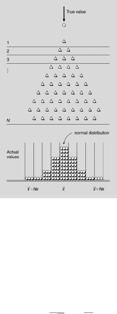
Francis Galton (1822-1911) devised a mechanical system called a quin-

cunx to demonstrate how the normal probability density function results

from a very large number of small eﬀects with each eﬀect having the same

probability of success or failure. This is illustrated in Figure 6.2. As a ball

enters the quincunx and encounters the ﬁrst eﬀect, it falls a lateral distance

e to either the right or the left. This event has caused it to depart slightly

from its true center. After it encounters the second event, it can either re-

turn to the center or depart a distance of 2e from it. This process continues

for a very large number, N, of events, resulting in a continuum of possible

outcomes ranging from a value of ¯x − Ne to a value of ¯x + N e. The key,

of course, to arrive at such a continuum of normally distributed values is

to have e small and N large. This illustrates why many phenomena are

normally distributed. In many situations there are a number of very small,

uncontrollable eﬀects always present that lead to this distribution.

6.3 Normalized Variables

For convenience in performing statistical calculations, the statistical variable

often is nondimensionalized. For any statistical variable x, its standardized

normal variate, β, is deﬁned by

β = (x − x

)/σ, (6.3)

in which x

is the mean value of the population and σ its standard devia-

tion. In essence, the dimensionless variable β signiﬁes how many standard

deviations that x is from its mean value. When a speciﬁc value of x, say x

is considered, the standardized normal variate is called the normalized z

variable, z

, as deﬁned by

= (x

− x

)/σ. (6.4)

These deﬁnitions can be incorporated into the probability expression of a

dimensional variable to yield the corresponding expression in terms of the

nondimensional variable. The probability that the dimensional variable x

will be in the interval x

± δx can be written as

P (x

− δx ≤ x ≤ x

+ δx) =

+δx

−δx

p(x)dx. (6.5)

Statistics 187

FIGURE 6.2

Galton’s quincunx.

Note that the width of the interval is 2δx, which in some previous expressions

was written as ∆x. Likewise,

P (−x

≤ x ≤ +x

) =

−x

p(x)dx. (6.6)

This general expression can be written speciﬁcally for a normally dis-

tributed variable as

P (−x

≤ x ≤ +x

) =

−x

√

2π

exp



−

2σ

(x − x

)



dx. (6.7)

188 Measurement and Data Analysis for Engineering and Science

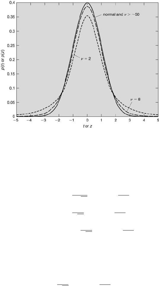
FIGURE 6.3

The normal and Student’s t probability density functions.

Using Equations 6.3 and 6.4 and noting that dx = σdβ, Equation 6.7 be-

comes

P (−z

≤ β ≤ +z

) =

√

2π

−z

exp



−β



σdβ,

√

2π

−z

exp



−β



dβ,

= 2



√

2π

exp



−β



dβ



. (6.8)

The factor of 2 in the last equation reﬂects the symmetry of the normal

probability density function, which is shown in Figure 6.3, in which p(z)

is plotted as a function of the normalized-z variable. The term in the { }

brackets is called the normal error function, denoted as p(z

). That is

p(z

) =

√

2π

exp



−β



dβ. (6.9)

The values of p(z

) are presented in Table 6.2 for various values of z

. For

example, there is a 34.13 % probability that a normally distributed variable

will be within the range from x

−x

= 0 to x

−x

= σ [p(z

) = 0.3413].

In other words, there is a 34.13 % probability that a normally distributed

Statistics 189

% P

68.27

1.645

90.00

1.960

95.00

95.45

2.576

99.00

99.73

99.99

TABLE 6.1

Probabilities of some common z

values.

variable will be within one standard deviation above the mean. Note that the

normal error function is one-sided because it represents the integral from 0

to +z

. Some normal error function tables are two-sided and represent the

integral from −z

to +z

. Always check to see whether such tables are either

one-sided or two-sided.

Using the deﬁnition of z

, the probability that a normally distributed

variable, x

, will have a value within the range x

± z

σ is

2p(z

) =

√

2π

exp



−



dβ =

% P

100

. (6.10)

In other words, there is P percent probability that the normally distributed

variable, x

, will be within ±z

standard deviations of the mean. This can

be expressed formally as

= x

± z

σ (% P ). (6.11)

The percent probabilities for the z

values from 1 to 4 are presented in

Table 6.1. As shown in the table, there is a 68.27 % chance that a normally

distributed variable will be within ± one standard deviation of the mean

and a 99.73 % chance that it will be within ± three standard deviations of

the mean.

Example Problem 6.1

Statement: Consider the situation in which a large number of voltage measurements

are made. From this data, the mean value of the voltage is 8.5 V and that its variance

is 2.25 V

. Determine the probability that a single voltage measurement will fall in the

interval between 10 V and 11.5 V. That is, determine Pr[10.0 ≤ x ≤ 11.5].

Solution: Using the deﬁnition of the probability distribution function, P r[10.0 ≤

x ≤ 11.5] = P r[8.5 ≤ x ≤ 11.5] − P r[8.5 ≤ x ≤ 10.0]. The two probabilities on the

right side of this equation are found by determining their corresponding normalized

z-variable values and then using Table 6.2.

First, P r[8.5 ≤ x ≤ 10.0]:

z =

x − x

10 − 8.5

1.5

= 1 ⇒ P (8.5 ≤ x ≤ 10.0) =

.6827

= 0.3413.

190 Measurement and Data Analysis for Engineering and Science

Then, P r[8.5 ≤ x ≤ 11.5]:

z =

11.5 − 8.5

1.5

= 2 ⇒ P (8.5 ≤ x ≤ 11.5) =

.9545

= 0.4772.

Thus, P r[10.0 ≤ x ≤ 11.5] = 0.4772 - 0.3413 = 0.1359 or 13.59 %. Likewise, the

probability that a single voltage measurement will fall in the interval between 10 V

and 13 V is 15.74 %.

Example Problem 6.2

Problem Statement: Based upon a large data base, the State Highway Patrol has

determined that the average speed of Friday-afternoon drivers on an interstate is 67

mph with a standard deviation of 4 mph. How many drivers out of 1000 travelling on

that interstate on Friday afternoon will be travelling in excess of 72 mph?

Problem Solution: Assume that the speeds of the drivers follow a normal distribu-

tion. The 72 mph speed ﬁrst converted into its corresponding z-variable value is

z =

72 − 67

= 1.2. (6.12)

Thus, we need to determine

P r[z > 1.2] = 1 − P r[z ≤ 1.2] = 1 − (P r[−∞ ≤ z ≤ 0] + P r[0 ≤ z ≤ 1.2]). (6.13)

From the one-sided z-variable probability table

P r[0 ≤ z ≤ 1.2] = 0.3849. (6.14)

Also, because the normal probability distribution is symmetric about its mean

P r[−∞ ≤ z ≤ 0] = 0.5000. (6.15)

Thus,

P r[z > 1.2] = 1 − (0.5000 + 0.3849) = 0.1151. (6.16)

This means that approximately 115 of the 1000 drivers will be travelling in excess of

72 mph on that Friday afternoon.

6.4 Student’s t Distribution

It was about 100 years ago that William Gosset, a statistician working for

the Guinness brewery, recognized a problem in using the normal distribu-

tion to describe the distribution of a small sample. As a consequence of his

observations it was recognized that the normal probability density function

overestimated the probabilities of the small-sample members near its mean

and underestimated the probabilities far away from its mean. Using his data

as a guide and working with the ratios of sample estimates, Gosset was able

to develop a new distribution that better described how the members of

a small sample drawn from a normal population were actually distributed.

Statistics 191

0.00 0.01 0.02 0.03 0.04 0.05 0.06 0.07 0.08 0.09

0.0 .0000 .0040 .0080 .0120 .0160 .0199 .0239 .0279 .0319 .0359

0.1 .0398 .0438 .0478 .0517 .0557 .0596 .0636 .0675 .0714 .0753

0.2 .0793 .0832 .0871 .0910 .0948 .0987 .1026 .1064 .1103 .1141

0.3 .1179 .1217 .1255 .1293 .1331 .1368 .1406 .1443 .1480 .1517

0.4 .1554 .1591 .1628 .1664 .1700 .1736 .1772 .1808 .1844 .1879

0.5 .1915 .1950 .1985 .2019 .2054 .2088 .2123 .2157 .2190 .2224

0.6 .2257 .2291 .2324 .2357 .2389 .2422 .2454 .2486 .2517 .2549

0.7 .2580 .2611 .2642 .2673 .2704 .2734 .2764 .2794 .2823 .2852

0.8 .2881 .2910 .2939 .2967 .2995 .3023 .3051 .3078 .3106 .3133

0.9 .3159 .3186 .3212 .3238 .3264 .3289 .3315 .3340 .3365 .3389

1.0 .3413 .3438 .3461 .3485 .3508 .3531 .3554 .3577 .3599 .3621

1.1 .3643 .3665 .3686 .3708 .3729 .3749 .3770 .3790 .3810 .3830

1.2 .3849 .3869 .3888 .3907 .3925 .3944 .3962 .3980 .3997 .4015

1.3 .4032 .4049 .4066 .4082 .4099 .4115 .4131 .4147 .4162 .4177

1.4 .4192 .4207 .4222 .4236 .4251 .4265 .4279 .4292 .4306 .4319

1.5 .4332 .4345 .4357 .4370 .4382 .4394 .4406 .4418 .4429 .4441

1.6 .4452 .4463 .4474 .4484 .4495 .4505 .4515 .4525 .4535 .4545

1.7 .4554 .4564 .4573 .4582 .4591 .4599 .4608 .4616 .4625 .4633

1.8 .4641 .4649 .4656 .4664 .4671 .4678 .4686 .4693 .4699 .4706

1.9 .4713 .4719 .4726 .4732 .4738 .4744 .4750 .4758 .4761 .4767

2.0 .4772 .4778 .4783 .4788 .4793 .4799 .4803 .4808 .4812 .4817

2.1 .4821 .4826 .4830 .4834 .4838 .4842 .4846 .4850 .4854 .4857

2.2 .4861 .4864 .4868 .4871 .4875 .4878 .4881 .4884 .4887 .4890

2.3 .4893 .4896 .4898 .4901 .4904 .4906 .4909 .4911 .4913 .4916

2.4 .4918 .4920 .4922 .4925 .4927 .4929 .4931 .4932 .4934 .4936

2.5 .4938 .4940 .4941 .4943 .4945 .4946 .4948 .4949 .4951 .4952

2.6 .4953 .4955 .4956 .4957 .4959 .4960 .4961 .4962 .4963 .4964

2.7 .4965 .4966 .4967 .4968 .4969 .4970 .4971 .4972 .4973 .4974

2.8 .4974 .4975 .4976 .4977 .4977 .4978 .4979 .4979 .4980 .4981

2.9 .4981 .4982 .4982 .4983 .4984 .4984 .4985 .4985 .4986 .4986

3.0 .4987 .4987 .4987 .4988 .4988 .4988 .4989 .4989 .4989 .4990

3.5 .4998 .4998 .4998 .4998 .4998 .4998 .4998 .4998 .4998 .4998

4.0 .5000 .5000 .5000 .5000 .5000 .5000 .5000 .5000 .5000 .5000

TABLE 6.2

Values of the normal error function.

192 Measurement and Data Analysis for Engineering and Science

Because his employer would not allow him to publish his ﬁndings, he pub-

lished them under the pseudonym “Student”[2]. His distribution was named

the Student’s t distribution. “Student” continued to publish signiﬁcant

works for over 30 years. Mr. Gosset did so well at Guinness that he eventu-

ally was put in charge of its entire Greater London operations [1].

The essence of what Gosset found is illustrated in Figure 6.3. The solid

curve indicates the normal probability density function values for various z.

It also represents the Student’s t probability density function for various t

and a large sample size (N > 100). The dashed curve shows the Student’s

t probability density function values for various t for a sample consisting

of 9 members (ν = 8), and the dotted curve for a sample of 3 members

(ν = 2). It is clear that as the sample size becomes smaller, the normal

probability density function near its mean (where z = 0) overestimates the

sample probabilities and, near its extremes (where z > ∼ 2 and z < ∼ −2),

underestimates the sample probabilities. These diﬀerences can be quantiﬁed

easily using the expressions for the probability density functions.

The probability density function of Student’s t distribution is

p(t, ν) =

Γ[(ν + 1)/2]

√

πνΓ(ν/2)



1 +



−(ν+1)/2

, (6.17)

where ν denotes the degrees of freedom and Γ is the gamma function, which

has these properties:

Γ(n) = (n − 1)! for n = whole integer

Γ(m) = (m − 1)(m − 2)...(3/2)(1/2)

√

π for m = half −integer

Γ(1/2) =

√

Note in particular that p = p(t, ν) and, consequently, that there are an

inﬁnite number of Student’s t probability density functions, one for each

value of ν. This was suggested already in Figure 6.3 in which there were

diﬀerent curves for each value of N.

The statistical concept of degrees of freedom was introduced by R.A.

Fisher in 1924 [1]. The number of degrees of freedom, ν, at any stage in

a statistical calculation equals the number of recorded data, N, minus the

number of diﬀerent, independent restrictions (constraints), c, used for the

required calculations. That is, ν = N − c. For example, when computing

the sample mean, there are no constraints (c = 0). This is because only the

actual sample values are required (hence, no constraints) to determine the

sample mean. So for this case, ν = N. However, when either the sample

standard deviation or the sample variance is computed, the value of the

sample mean value is required (one constraint). Hence, for this case, ν =

N − 1. Because both the sample mean and sample variance are contained

implicitly in t in Equation 6.17, ν = N −1. Usually, whenever a probability

density function expression is used, values of the mean and the variance are

required. Thus, ν = N −1 for these types of statistical calculations.

Statistics 193

The expressions for the mean and standard deviation were developed in

Chapter 5 for a continuous random variable. Analogous expressions can

be developed for a discrete random variable. When N is very large,

= lim

N→∞

i=1

(6.18)

and

= lim

N→∞

i=1

− x

)

. (6.19)

When N is small,

¯x =

i=1

(6.20)

and

N − 1

i=1

− ¯x)

. (6.21)

Here ¯x denotes the sample mean, whose value can (and usually does) vary

from that of the true mean, x

. Likewise, S

denotes the sample variance

in contrast to the true variance σ

. The factor N − 1 occurs in Equation

6.21 as opposed to N to account for loosing one degree of freedom (¯x is

needed to calculate S

Example Problem 6.3

Statement: Consider an experiment in which a ﬁnite sample of 19 values of a

pressure are recorded. These are in units of kPa: 4.97, 4.92, 4.93, 5.00, 4.98, 4.92, 4.91,

5.06, 5.01, 4.98, 4.97, 5.02, 4.92, 4.94, 4.98, 4.99, 4.92, 5.04, and 5.00. Estimate the

range of pressure within which another pressure measurement would be at P = 95 %

given the recorded values.

Solution: From this data, using the equations for the sample mean and the sample

variance for small N,

¯p =

i=1

= 4.97 and S

19 − 1

i=1

− ¯p)

= 0.046.

Now ν = N − 1 = 18, which gives t

ν,P

= t

18,95

= 2.101 using Table 6.4. So,

= ¯p ± t

ν,P

(% P ) ⇒ p

= 4.97 ± 0.10 (95 %)

Thus, the next pressure measurement is estimated to be within the range of 4.87 kPa

to 5.07 kPa at 95 % conﬁdence.

Now, what if the sample had the same mean and standard deviation values but

they were determined from only ﬁve measurements? Then

ν,P

= t

4,95

= 2.770 ⇒ p

= 4.97 ± 0.13 (95 %)

194 Measurement and Data Analysis for Engineering and Science

ν,P

ν=2

ν=8

ν=100

57.74

65.34

68.03

81.65

91.95

95.18

90.45

98.29

99.66

94.28

99.61

99.99

TABLE 6.3

Probabilities for some typical t

ν,P

values.

For this case the next pressure measurement is estimated to be within the range of 4.84

kPa to 5.10 kPa at 95 % conﬁdence. So, for the same conﬁdence, a smaller sample size

implies a broader range of uncertainty.

Further, what if the original sample size was used but only 50 % conﬁdence was

required in the estimate? Then

ν,P

= t

18,50

= 0.668 ⇒ p

= 4.97 ± 0.03 (50 %)

For this case the next pressure measurement is estimated to be within the range of 4.94

kPa to 5.00 kPa at 50 % conﬁdence. Thus, for the same sample size but a lower required

conﬁdence, the uncertainty range is narrower. On the contrary, if 100 % conﬁdence was

required in the estimate, the range would have to extend over all possible values.

In a manner analogous to the method for the normalized z variable in

Equation 6.4, Student’s t variable is deﬁned as

= (x

− ¯x)/S

. (6.22)

It follows that the normally distributed variable x

in a small sample will

be within ±t

ν,P

sample standard deviations from the sample mean with %

P conﬁdence. This can be expressed formally as

= ¯x ± t

ν,P

(% P ). (6.23)

The interval ±t

ν,P

is called the precision interval. The percentage prob-

abilities for the t

ν,P

values of 1, 2, 3, and 4 for three diﬀerent values of ν

are shown in Table 6.3. Thus, in a sample of nine (ν = N − 1 = 8), there

is a 65.34 % chance that a normally distributed variable will be within ±

one sample standard deviation from the sample mean and a 99.61 % chance

that it will be within ± four sample standard deviations from the sample

mean. Also, as the sample size becomes smaller, the percent P that a sam-

ple value will be within ± a certain number of sample standard deviations

becomes less. This is because Student’s t probability density function is

slightly broader than the normal probability density function and extends

out to larger values of t from the mean for smaller values of ν, as shown in

Figure 6.3.

Statistics 195

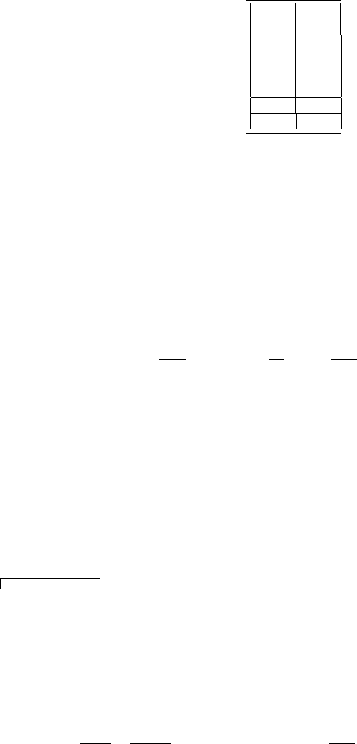
1 %

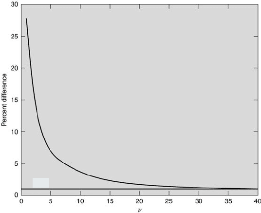
FIGURE 6.4

Comparison of Student’s t and normal probabilities.

Another way to compare the Student’s t distribution with the normal

distribution is to examine the percent diﬀerence in the areas underneath

their probability density functions for the same range of z and t values.

This implicitly compares their probabilities, which can be done for various

degrees of freedom. The results of such a comparison are shown in Figure

6.4. The probabilities are compared between t and z equal to 0 up to t

and z equal to 5. It can be seen that the percent diﬀerence decreases as the

number of degrees of freedom increases. At ν = 40, the diﬀerence is less than

1 %. That is, the areas under their probability density functions over the

speciﬁed range diﬀer by less than 1 % when the number of measurements

are approximately greater than 40.

The values for t

ν,P

are given in Table 6.4. Using this table, for ν = 8

there is a 95 % probability that a sample value will be within ±2.306 sample

standard deviations of the sample mean. Likewise, for ν = 40, there is a 95

% probability that a sample value will be within ±2.021 sample standard

deviations of the sample mean.

A relationship between Student’s t variable and the normalized-z vari-

able can be found directly by equating the x

s of Equations 6.11 and 6.23.