Peube J-L. Fundamentals of fluid mechanics and transport phenomena

Подождите немного. Документ загружается.

462 Fundamentals of Fluid Mechanics and Transport Phenomena



[8.87]

This equation is of a form analogous to [8.86] where the differentiation operators

are separated into two parts, the time derivative constitutes the perturbation term.

The calculation is performed as before and we seek a series development of

functions in separated variables:

 

KWWHKT

[8.88]

Letting

 , equation [8.87] can be written:

We obtain the recurrence relations:

 

   

!!!!

WWWKK

1212

0101



iiii

ggffM

TgfM

[8.89]

which are associated with the boundary conditions:

       

f f f ,,2,100;10;,,2,1,00

!! iffif

Taking account of the conditions at infinity, the function f

(

) is (see section

5.4.5.4):



erff  1

The analytical calculation of the functions f

is difficult: even if the solution to

the homogenous equation



fM can be expressed easily as a function of a

multiplicative constant (section 5.4.5.4), the variation of constants method is

impractical on account of the complexity of calculations. A numerical solution,

Thermal Systems and Models 463

which is preferable, makes the easy calculation of the first functions f

possible. The

series of functions f

is alternated and tends asymptotically to two functions equal to



r f which can be easily determined from system [8.89]:

  

with: 0 0Mf f f f

dd d d

  d 

The reader can verify that we have:



exp( ) ( : constant)f  c c



However, the recurrence relation

 

WWW

1

does not provide a simple

expression for the functions g

. Furthermore, we note that the perturbation term

ww of equation [8.87], of order

 

tTtT

in relative value, must remain

quite small: the temporal derivative of the imposed temperature must decay quickly

enough as time increases. From a physical point of view, it seems natural that in

order to remain as a small perturbation, the imposed temperature variation decreases

with time as the temperature distribution of the base solution T

spreads (Figure

8.6). In order to render the perturbation uniform in time, we compress the time scale

by performing the temporal variable change:







gtGt



which simplifies recurrence relation [8.89] of the functions g

, which can be written:

      

  

!!!!!!!!!

tTtGtG

tTtGtGtTtGtTtG

wii

www

ˆˆˆ

ˆˆˆˆˆˆˆ

)(



[8.90]

The parametric expression of the solutions for the thermal shock is thus:



)(

ftTtxT

[8.91]

The derivatives of the function T

(t) being taken with respect to the variable

tt ln

The thermal flux density at the wall can be written:





)(

ftT

464 Fundamentals of Fluid Mechanics and Transport Phenomena

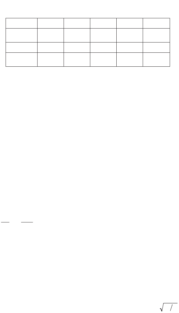
The values of the derivative



are shown in Table 8.2.

i 0 1 2 3 4

2/)0(

–0.5642 –0.7821 0.3859 –0.3203 0.2985

i 5 6 7 8 9

2/)0(

–0.2897 0.2857 –0.2838 0.2829 –0.2826

Table 8.2.

Values of the derivative



The preceding method can also be applied to the expression of solutions in the

vicinity of the base solutions of the form



. In particular, it is easy to verify

that the value n = 1/2 corresponds to the constant thermal flux which is given at the

wall. The solutions where the thermal flux varies gradually can be obtained as

before.

8.5.3.3.

Harmonic solutions of the equations for continuous media

The method described in section 8.5.2.4 can be applied to continuous media by

eliminating the temporal variable of the partial differential equation of the problem.

Let us take the example of temperature oscillation applied to the surface of abscissa

x = 0 of a semi-infinite wall. We encounter this problem of oscillatory thermal

penetration into rocks or ground which is subjected to daily or annual temperature

variations. Assuming a homogenous medium, the temperature



txT , satisfies heat

equation [8.32] with the following boundary conditions:

  

,;cos,0; TtTtTtT

f4

[8.92]

We seek solutions of the form:



xfeTT

4 

The heat equation becomes a differential equation:



xaffj ''

whose characteristic equation (



jra ) has roots:



ajr 2/1 r .

Thermal Systems and Models 465

The real solutions sought for the temperature distribution can be written:



xtxTT 4  cosexp

The depth

a2 is a space constant for the thermal damping oscillation.

The solution represents a temperature oscillation which becomes damped with

increasing depth. A numerical application shows that this damping is fast: taking a

value of 10

-6

-1

for the thermal diffusivity of the ground (corresponding to an

average rock), we find that

is respectively equal to 0.17 meters and to 3.15 meters

for daily and annual oscillations of temperature. The oscillation phase is opposite at

a depth of

/2 where amplitude has been reduced by a factor equal to 1.65.

The complex amplitudes method can be applied equally well to problems defined

in finite domains (walls, cylinders, etc.).

8.6. Model reduction

8.6.1. Overview

The objective of a knowledge model is to capture the evolution of a system, the

sub-system interactions of which we do not know. It comprises a large number of

variables in order to represent all the possible properties. The results involve either a

large quantity of numerical results from a computer solution or analytical

representations which may be more or less complex. The use of a knowledge model

amounts to performing a numerical experiment, which is often less expensive than a

physical experiment. A model is often too complex for a simple description of a

particular category of evolutions. Reduction of this model consists of replacing it

with a reduced model having a smaller number of variables, and whose objective is

to represent the principal phenomena with regard to the objective which is defined

(physical understanding of the model mechanisms, elaboration of a simulation

program or engineering formulae, control of processes). We are therefore interested

in decomposing the system into a small number of components with relatively

simple properties and whose interactions can provide a representative description of

the system in fixed conditions. Of course, the reduced model is not adapted to the

study of other operating conditions in the system.

Model reductions can be performed using various methods. However, the value

of the results of a model or of an experiment always depends on the pertinence of the

original hypotheses, on the reasoned use of numerical solutions or physical

measurement techniques and on a suitable physical analysis of the phenomena.

Certain methods consist of the performance of a numerical solution of a system by

means of a knowledge model, and the coupling of inputs and outputs with

466 Fundamentals of Fluid Mechanics and Transport Phenomena

representations of an empirical form which can be obtained by least mean square

methods; this practice has been used for a long time in order to establish engineering

formulae for certain applications. It has evolved into more sophisticated forms

through the use of more sophisticated mathematical methods. The use of these

methods is only justified as a method of exploiting the calculations resulting from a

physical analysis, which evaluates the nature of the approximations that are made

and the relative importance of the components in the functioning of a system. We

will prefer methods which increase our physical knowledge of the system studied,

and we will assume that the variables of the knowledge model have a physical

meaning and are not simply numerical values collected from experiments.

8.6.2. Model reduction of discrete systems

8.6.2.1. Principles of reduction of the state representation

A knowledge model, in the form of a state representation of a system with n state

variables or of an equivalent representation (an nth order differential equation in one

variable, etc.) makes the detailed description of all possible evolutions of the system.

The complexity associated with a large number n of variables leads to it being

replaced by a model with s state variables (s < n), called a reduced model, the

objective of which is to represent a particular evolution of the given physical system

(including its inputs and outputs) with good accuracy, or more general evolutions

with reduced precision. We have already seen some examples in section 8.3.2.2.3.

By definition, a differential system of order s cannot be equivalent to a

differential system of order n (n > s); however, these systems may have an identical

behavior for a family of solutions which depend on at most s parameters. The

reduction in the number of variables appearing in the differential equations can only

come from a regrouping of the equations, allowing the replacement of several

variables by a single variable or simplification of the equations, which lose their

differential character. Consider knowledge model [8.93]:

XDYUBXA

... 

[8.93]

Consider the reduced state vector X

with s components (s < n) derived from X

by a passage matrix R from X to X

= R X); the state vector X

satisfies the

reduced state representation:

rrrrr

XDYUBXA

 ..

[8.94]

with conditions [8.95] obtained by multiplying the left-hand side of equation [8.93]

by R and by comparing with [8.94]:

Thermal Systems and Models 467

 

.00;; DRDRXXRBBRARA

rrrr

[8.95]

If conditions [8.95] are exactly satisfied, representation [8.94] is an exact

reduced model for the ensemble of solutions X of [8.93] such that RX is non-zero.

However, in general, with the exception of cases where these solutions are known

explicitly, the realization of an exact reduced model is impractical.

Assuming conditions [8.95] are not satisfied, reduced representation [8.94] is an

approximate reduced model. The reduced vector X

= RX of the solution X of [8.93],

does not exactly satisfy equation [8.94]; if q is the residuum, the error of equation

[8.94]:

qUBXA

rrr

 ..

[8.96]

Let

be a solution of [8.94]:

UBXA

rrr



[8.97]

We define the error

XXe



with respect to the exact solution

assumed

to be verified by equation [8.94]; it satisfies the differential equation obtained by

subtracting term by term [8.96] and [8.97]:

UBXA

eAqeA

rrr

..  

We must therefore determine the matrices R, A

and B

, such that the error of

equation q is minimized. This minimization procedure can be performed on an

ensemble of known solutions. We will leave aside the details of this kind of

procedure.

It is easy to impose that the reduction be exact for the steady regime. In this case,

equations [8.93] and [8.94] can be solved and we obtain:

BURARXUBAX

rrr



 

and consequently the relation:

BRAAB

1

In the unsteady regime, the preceding elimination is no longer possible and the

vector RX obtained with the solution of [8.93] is no longer equal to the solution

468 Fundamentals of Fluid Mechanics and Transport Phenomena

of [8.97]. The matrix A

can be determined by minimizing the error of equation q.

This minimization can be performed for chosen inputs and for criteria which need to

be defined for the weighting to be applied at different instants [PET 91]. This

procedure comes down to performing a numerical interpolation on the knowledge

model by means of a reduced model.

8.6.2.2.

Physical aspects of the model reduction

The considerations of the preceding section are essentially of a mathematical

nature and they leave a wide choice for the variables (in particular the matrix R), the

class of solutions and the objectives of error minimization. They can be applied to a

perfect knowledge model from the perspective of thermodynamics (sub-systems in

quasi-equilibrium), this needing to be verified for solutions which vary quite slowly

in space-time. The reduction in a knowledge model can only have a limited interest

if the discretization is too rough in certain domains. The partitioning of a system into

sub-systems is the most important operation and we will assume that it is suitable. In

general, the reduction in the number of variables is associated with a regrouping of

components, which leads to a choice of the reduced variables to be retained; this

should be done such that the definition of the mean intensive variables of the sub-

systems of the reduced model have a reasonable physical meaning in the balance

equations (section 1.4.2.5 and section 6.5.2.4).

The grouping of sub-systems which are in neighboring or identical states leads to

the replacement of many differential equations by a single equation: for example, a

material domain which has been segmented into three components and whose

temperatures are close can be represented by a single component at a suitable

temperature whose thermal energy is the sum of the energies of the components.

The sub-systems whose extensive quantity contents are small can often be

eliminated or assimilated into neighboring components, leading to the suppression

of the corresponding variables. The components whose extensive quantities are

constant or vary little can become sources of established fluxes: they thus play a role

of a simple resistance for the transfer of extensive quantities and their modeling

loses its differential character. We have seen two examples in sections 8.3.1.3 and

8.3.1.4.

In general, the number and the size of the sub-systems (or the grid of the system

domain) must be adapted to the categories of the solutions studied. Let us take the

example of the discretization on a continuous medium of a wall whose surfaces are

subjected to a thermal shock (section 8.3.2.2.2). Let us begin by segmenting the wall

into 50 equal elements in series (a system analogous to that of section 8.3.1.3).

Figure 8.13 shows that the temperature variations in the first instances are rapid in

the vicinity of the wall surface, whereas later, they become quite regular. The

discretization in equal elements is thus not the best solution: a finer discretization is

Thermal Systems and Models 469

needed in the vicinity of the wall surfaces if we want to have a suitable precision in

the first instants, whereas such a fine discretization is not necessary later in the

central part of the wall. A better result with 50 elements is obtained when these are

distributed broadly at the center of the wall, and extremely close to the edges of the

wall.

8.6.2.3.

The problem of local constraints

However, many systems present local constraints (in the mathematical sense) on

certain intensive variables related to the possible modification of material elements:

deteriorations due to excessive temperature or to large

instantaneous stresses. In

this case, we obviously cannot eliminate from the model the small component which

contains, for example, a small thermal energy, but which possesses a critical

temperature value (temperature of a thermal measurement probe, a fragile element

whose temperature must be limited, etc.). The intensive variable concerned (often

the local temperature) is necessary for the regulation of a controller whose job it is

to modify or stop the system functioning. Model reduction in such zones is

obviously delicate.

8.6.2.4.

Modal reduction of time-invariant linear systems

8.6.2.4.1.

Introduction

Modal reduction is essentially concerned with time-invariant linear systems

whose transitional solution is the sum of eigenmodes of the system of equations (see

the examples of discrete or continuous systems in section 8.3). The solution of a

linear system can be expressed in an explicit modal form using initial conditions and

an established solution (section 8.2.2.2); the reduction here amounts to a

simplification operation, but the question regarding the pertinence of the different

modes arises for discretized systems. We are then interested in writing a reduced

state representation which will allow the numerical simulation of the system in

complex conditions.

8.6.2.4.2.

Modal reduction of continuous solution of continuous media

The modal solution of the heat equation involves replacing the continuous

variable by a denumerable set of mode coefficients in the explicit expression of

solution [8.38] in the form of a series. The reduction problem therefore consists of

simplifying and/or truncating this series. A consequence of this truncation is the

introduction of a discontinuity at the time origin, which amounts to assuming that

For example, cavitation (vaporization and chiefly sudden condensation) when local pressure

in a liquid flow is less than the saturation vapor pressure, high temperature on a wall in high

supersonic or hypersonic air flow, production of pollutants inside engines or chemical

reactors due to local bad conditions of temperature or concentrations, etc.

470 Fundamentals of Fluid Mechanics and Transport Phenomena

fast energy transfers in the higher order modes occur instantaneously (section

8.2.2.2). Various authors avoid this discontinuity by adding a fictitious mode or by

attributing to the last mode retained the total remaining amplitude. Let us illustrate

this problem by reconsidering the example of thermal shock on the wall edges

(section 8.3.2.2.2).

(t)

1 20

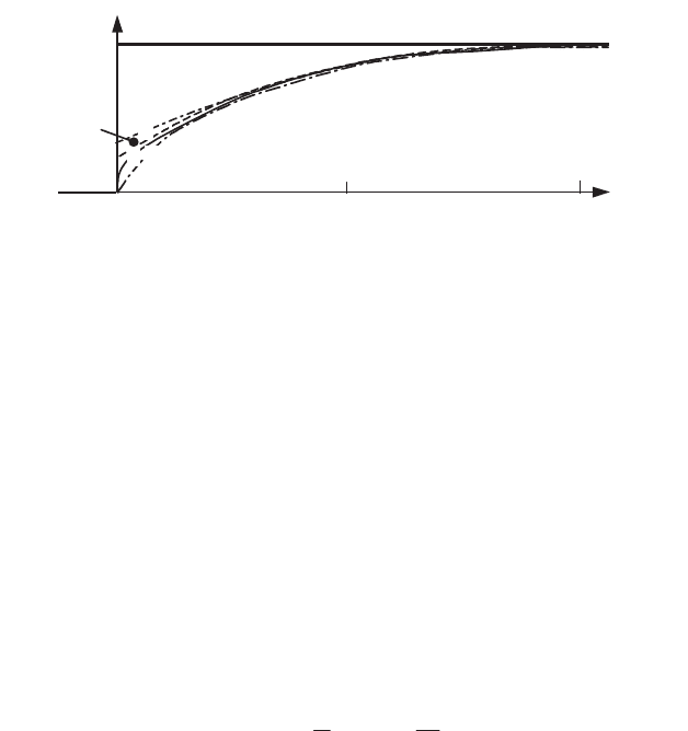
Figure 8.17.

Mean temperature on a wall during a thermal shock on its two faces

(section 8.3.2.2.2). The draughts are indicative

Let us consider the mean temperature T

(formula [8.41]), which translates the

thermal energy evolution over the course of the heating processes caused by the

thermal shock (curve 1, Figure 8.17). We have seen (Table 8.1) that the first mode

contains 81% of the process energy; in only conserving this first mode, we obtain a

representation for the temperature T

(curve 2, Figure 8.17), which contains a

discontinuity at the origin equal to



019.TT ; considering the first two modes of

the series representing T

(curve 3, Figure 8.17) this discontinuity is reduced to



010.TT ).

We can remove this discontinuity by including the total remaining amplitude

(0.19 in relative units) in the highest mode retained (curve 4, Figure 8.17) in

accordance with the formula:



101

081 019

T(t) T T T [ . . ]



 





However, the second mode is now too large; we can therefore look to determine

a time constant of the second mode in order to achieve a better representation of the

function

(t), for example by a mean square error minimization method. It is also

possible to add a fictitious mode. It is clear that a good solution is not achieved and

the values obtained by empirical adjustments are not physically pertinent.

Thermal Systems and Models 471

In effect, in the first instants of the evolution, only zones in the vicinity of edges

are concerned with the heat transfer. Further from these, the sum of the series terms

[8.41] is zero:

the modal representation is not adapted to the representation of a

thermal boundary layer problem

(section 8.3.2.2.2). We can obviously note that the

thermal boundary layer is independent of the wall thickness

that can take any

value: defining modes by means of an arbitrary length is indeed an irrational method

which cannot lead to a judicious mathematical representation.

A good reduced model of thermal conduction in a wall must also take into

account the modal aspect as the evolution of the unsteady boundary layer. There is

no other (or nearly no other) way to obtain such a reduced model than

a composite

representation

matching the modal representation and the thermal shock solution:

we have presented this method in section 8.3.2.2.3, where a good precision was

obtained for the mean temperature [8.46], using only the first mode. This method

also has the advantage of giving precise values for the thermal flux density at the

edges [8.47] at any instant.

8.6.2.4.3.

Modal reduction of discrete models

In section 8.6.2.2 we considered the model with 50 elements of a continuous

wall subjected to a thermal shock, leading to a linear system with 50 variables, and

which thus comprises 50 eigenvalues and eigenmodes. We will consider that a half

period of a sinusoid requires at least ten intervals in order to be represented by a

constant function in each element. The interval under study cannot therefore

comprise more than five arches: we can only represent the first three even modes

and the first two odd modes (see Figure 8.12). The 45 other modes are increasingly

noisy as the order is increased (the 50

mode corresponds to a change of sign of the

eigenfunction between each of the 50 intervals). Their physical existence is

increasingly problematic and it is not useful to consider them despite the fact that

they constitute exact solutions of the model.

A discretization into sub-systems should comprise a sufficiently large number of

elements, but only a few modes are actually useful

. The modal solution is obviously

the most interesting because it provides a structured knowledge which highlights the

system properties. However, the discretization of a linear system proceeding from

the calculation of its modes requires more elements than a discretization, taking into

account physical aspects and particularly the level of unbalance between two

neighboring sub-systems: if we consider the preceding example of the wall on the

interval [-1,+1], it is necessary to calculate the modes to be retained over the entire

interval, whose form (Figure 8.12) requires discretization of the interval [-1,+1] in

equal segments, as opposed to a numerical resolution for which a discretization,

narrower near the wall faces and wider in the central part, is more fitted to the form