Roy K.K. Potential theory in applied geophysics
Подождите немного. Документ загружается.

13.6 Oscillating Vertical Magnetic Dipole Placed on the Surface of the Earth 399
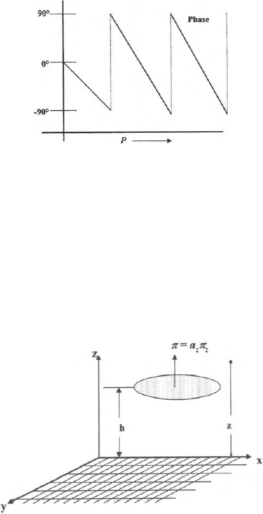
Fig. 13.8. Variation of phase of H
ψ
13.6 Electromagnetic Field due to an Oscillating Vertical
Magnetic Dipole Placed on the Surface of the Earth
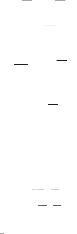
A coil carrying current is a magnetic dipole. It generates the magnetic field
around the coil (Fig. 13.9). When an alternating current is sent through the
same coil, it becomes an oscilla tin g magnetic dipole and electromagnetic waves
start propagating in all the directions from this magnetic dipole. It is termed
as the vertical oscillating magnetic dipole when the plane of the coil is hori-
zontal and the magnetic field vector is vertical. When the plane of the coil is
vertical and the magnetic field vector is at right angles to the plane of coil i.e.,
horizontal, it is termed as the horizontal magnetic dipole (See next section)
Fig. 13.9. Vertical oscillating magnetic dipole on the surface of a homogenous earth

400 13 Electromagnetic Wave Propagation
In this problem, both the coil and the point of observation are initially
assumed to be in the air. They are finally brought down to the surface of the
earth to have a simplified solution to the problem. However, researchers can
introduce further complexities in the problem and arrive at a more general
solution taking this solution as a starting point. The simplest problems are
presented in this section. Many problems in this series have alre ady been
solved and they are available in published literatures. The problem due to
an oscillating magnetic dipole z is solved using Fitzeral d vector potential
F. From Sect. (13.2) we have seen that the expression for vector potential
at a distance r due to an oscillating electric dipole is
Π=
be
−γr
r
. Similarly
we have written the expression for the source potential for vertical magnetic
dipole as
F=m.
e
−γr
r
(13.103)
where m is the moment of the di pol e. For electric dipole
m=a
l
Il
4π(σ +iω ∈)
(13.104)
and for magnetic dipole
m=a
n
IS
4π
(13.105)
where S is the surface area of the current carrying coil. a
l
and a
n
are resp ec-
tively the unit vectors. Our problem is to find out the field s at any point
either outside o r on the surface of the earth. Moment of the vertical magnetic
dipole is directed normal to the boundary. The boundary plane is the air earth
boundary and the oscillating dipole is placed at a height ‘h’ from the surface.
The magnetic dipoles are taken along the z direction and are represented by
the Fitzerald vector
F. Basic structures of this type of boundary value prob-
lems are more or less the same with some problem dependent variations in
finer details.
This type of boundary value problems start with electromagnetic wave
equations. The Laplacian operator, to b e used, varies from source to source
of the electromagnetic waves. The problem can be solved either in
Eand
H
field domain as done in Sect. 13.1 or in vector potential domain as shown in
Sect. 13.2 to 13.8. The EM wave partial differential equations are solved using
the method of separation of variables. Once potential problems are solved in
a vector potential domain, one can obtain the electric and magnetic fields
using the appropriate relations between vector potentials and
Eand
Hfields
((13.72) to (13.74) and (13.76) to (13.77)). These relations are connectors
between
Eand
Hfieldwith
Πor
For
Aandφ,asdiscussedintheprevi-
ous chapter. In the (
A, φ) formulation φ is a scalar potential. At this stage
one has to find out the vanishing and non-vanishing components of the
E
and
H fields.Physics and geometry of the problems help in determining the
zero and non-zero c omp onents of the EM fields. The source potential and

13.6 Oscillating Vertical Magnetic Dipole Placed on the Surface of the Earth 401
the perturbation potentials are determined. They are brought to the same
form before the boundary conditions are applied. This step is more or less
the same as those used for potential field p roblems in direct current problem.
Bringing source potential and perturbation potential in the same form may
turn out to be a fairly complex mathematical problem. These arbitrary coef-
ficients, obtained while computing the perturbation p otentials by so lv i n g the
wave equation by method of separation of variables, are determined applying
boundary conditions. The final expressions for
Eand
H fields are obtained
either a nalytically or numerically depending up on the level of complexities in
mathematics.
The Fitzerald vector
F is directed along the z direction.
F=a
z
.
IS
4π
.
e
−γr
r
. (13.106)
In view of the cylindrical symmetry, the field
F
z
=f(ρ, z). (13.107)
Therefore, the Helmholtz wave equation
∇
2
F
z
= γ
2
F
z
(13.108)
reduces to
∂
2
F
z
∂ρ
2
+
1
ρ
∂F
z
∂ρ
+
∂
2
F
z
∂z
2
= γ
2
F
z
(13.109)
In this problem
F
ψ
=0and
∂
∂ψ
=0,whereψ is the azimuthal angle.
Now applying the method of separation of variables
F=R(ρ)Z(z) (13.110)
we get
1
R
d
2
R
dρ
2
+
1
ρR
.
dR
dρ
= −
1
Z
d
2
Z
dz
2
+ γ
2
. (13.111)
If we substitute
1
Z
d
2
Z
dz
2
= γ
2
+n
2
(13.112)
(13.111) reduces to
1
R
.
d
2
R
dρ
2
+
1
ρR
.
dR
dρ
+n
2
=0. (13.113)
The solutions of the first and second equations are respectively given by
(i)e
±
γ
2
+n
2
Z
and
(ii)J
0
(nρ)andY
0
(n
ρ
) (13.114)
402 13 Electromagnetic Wave Propagation
where J
0
and Y
0
are the Bessel’s function of first and second kind and of zero
order. The solutions of the vector potentials in the two media are
F
0
=
α
0
A
0
e
−Z
√
γ
2
+n
2
+B
0
e
+Z
√
γ
2
+n
2
J
0
(nρ)dn (13.115)
and
F
1
=
α
0
B
1
e
+z
√
γ
2
+n
2
J
0
(nρ)dn. (13.116)
Since Y
0
tends to infinity as r → 0, Y
0
cannot be present in the solution of the
problem.
F
0
in the first medium, will contain the source p otential. Therefore
F
0
=
me
−γ
0
r
r
+
α
0
A
n
e
−Z
√
γ
2
0
+n
2
J
0
(nρ)dn. (13.117)
B
n
cannot be present in the expression because the field must vanish at
infinite distance. In the second medium Z is assumed to be negative. The
vector potential should die down with depth in the absence of any kind of
reflector. Therefore
F
1
=
α
0
B
n
e
+Z
√
γ
2
1
+n
2
J
0
(nρ)dn. (13.118)
The connecting link between the Fitzerald vector and the electric and mag-
netic fields are respectively given by
E=−iωµ curl
F (13.119)
H=−γ
2
F + grad div
F
= curlcurl
F (13.120)
= −
1
iωµ
curl
E. (13.121)
In cylindrical coordinate system
curl
F=a
ρ
1
ρ
∂
F
z
∂ρ
−
∂
F
ψ
∂z
+ a
ψ
∂
F
ρ
∂z
−
∂
F
z
∂ρ
+ a
z
1
ρ
∂
∂ρ
(ρF
ψ
) −
1
ρ
∂F
ρ
∂ψ
. (13.122)
In this problem
∂
∂φ
=0,
E
p
=
E
z
=
H
ψ
=0and
13.6 Oscillating Vertical Magnetic Dipole Placed on the Surface of the Earth 403
E
ψ
=iωµ
∂F
z
∂ρ
(13.123)
H
ρ
=
1
iωµ
∂
E
ψ
∂Z
=
∂
∂Z
∂
F
∂ρ
(13.124)
Hz =
1
ρ
∂
∂ρ
ρ
∂
F
z
∂ρ
. (13.125)
Boundary conditions are
(E
ψ
)
0
=(E
ψ
)
1
(H
ρ
)
0
=(H
ρ
)
1
(13.126)
Therefore,
iωµ
0
∂F
∂ρ
0
=iωµ
1
∂F
∂ρ
1
and
∂
∂Z
.
∂F
∂ρ
0
=
∂
∂Z
∂F
∂ρ
1
. (13.127)
If a function is continuous across the boundary
µ
0
F
0
= µ
1
F
1
∂F
0
∂Z
=
∂F
1
∂Z
. (13.128)
These are the two sets of boundary conditions in this problem.
Weber Lipschitz integral
1
r
=
1
ρ
2
+z
2
=
α
0
e
−nZ
J
0
(nρ)dn (13.129)
has already been used in direct current field problem to convert the p oten-
tial function
1
r
in the form of an integral involvi n g Bessel’s function to bring
parity between the source potential and the perturbation potential. This is
an essential step for all electrical and electromag netic boundary value prob-
lems. For a time varying electromagnetic field Sommerfeld suggested the
formula
e
−γ
√
ρ
2
+z
2
ρ
2
+z
2
=
α
0
e
−Z
√
γ
2
+n
2
.
n
n
2
+ γ
2
.J
0
(nρ)dn. (13.130)
For γ = 0, i.e. for zero frequency, Sommerfeld’s formula reduces down to the
Web er’s formula. ‘r’ is always positive irrespective of the position of the point
of observation with respect to the ground and the transmitting antenna i.e.,
404 13 Electromagnetic Wave Propagation
r
2
= ρ
2
+(h− z)
2
or
ρ
2
+(z− h)
2
is always positive whether h is greater o r less than z.
Sommerfeld formula for this problem is
e
−γ
√
ρ
2
+(z−h)
2
ρ
2
+(z− h)
2
=
α
0
e
−|z−h|
√
γ
2
+n
2
.
n
n
2
+ γ
2
. (13.131)
The vector potentials in the two media now be written as
F
0
=m
α
0
e
−|z−h|
√
γ
2
0
+n
2
.
n
γ
2
0
+n
2
.J
0
(nρ)dn
+
α
0
A
n
e
−Z
√
γ
2
0
+n
2
J
0
(nρ)dn (13.132)
and
F
1
=
α
0
B
n
e
Z
√
γ
2
1
+n
2
.J
0
(nρ)dn. (13.133)
Applying the boundary conditions at z = 0, we get
µ
0
m
α
0
n
n
2
+ γ
2
0
e
−h
√
γ
2
0
+n
2
J
0
(nρ)dn
+ µ
0
α
0
A
n
J
0
(nρ)dn=µ
1
α
0
B
n
J
0
(nρ)dn (13.134)
⇒ µ
0
m.
n
n
2
+ γ
2
0
γ
2
0
+n
2
.e
−h
√
γ
2
0
+n
2
− µ
0
A
n
γ
2
0
+n
2
= µ
1
.B
n
γ
2
1
+n
2
.
(13.135)
From these two equations, we get the value of A
n
as
A
n
=m.
n
γ
2
0
+n
2
.
γ
2
0
+n
2
−
γ
2
1
+n
2
γ
2
0
+n
2
+
γ
2
1
+n
2
e
−n
√
γ
2
0
+n
2
. (13.136)
Now let
n
2
+ γ
2
0
=n
2
0
n
2
+ γ
2
1
=n
2
1
.
13.6 Oscillating Vertical Magnetic Dipole Placed on the Surface of the Earth 405
Then the (14.134, 14.135) simplify down to
µ
0
m
n
n
0
e
−n
0
h
+ µ
0
A
n
= µ
1
B
n
(13.137)
m
n
n
0
.e
−n
0
h
− n
0
A
n
=n
1
B
n
. (13.138)
From these two equations, the values of A
n
and B
n
comes out to be
A
n
=m.
n
n
0
.
Pn
0
− n
1
Pn
0
+n
1
e
−n
0
h
(13.139)
B
n
=m.
2n
1
Pn
0
+n
1
.e
−n
0
h
(13.140)
where
ρ =
µ
µ
0
.
Therefore the vector potentials in the two media are
F
0
=m
α
0
n
n
2
+ γ
2
0
.e
−|z−h|
√
γ
2
0
+n
2
J
0
(nρ)dn
+m
α
0
n
n
0
Pn
0
− n
1
Pn
0
+n
1
.e
−n
0
(z+h)
J
0
(nρ)dn (13.141)
and
F
1
=m
α
0
2n
Pn
0
+n
1
.e
−n
0
h+n
1
z
J
0
(nρ)dn. (13.142)
The
F
0
can be rewritten as
F
0
=m
α
0
n
n
0
.e
−|h−z|n
0
.J
0
(nρ)dn
+m
α
0
n
n
0
e
−n
0
(z+h)
J
0
(nρ)dn
− m
α
0
n
n
0
.
2n
1
Pn
0
+n
1
.e
−n
0
(z+h)
.J
0
(nρ)dn. (13.143)
This is equivalent to
me
−γ
0
r
r
+
me
−γ
0
r
1
r
1
− P
′
(13.144)
where
r=
ρ
2
+(z− h)
2
406 13 Electromagnetic Wave Propagation
r
1
=
ρ
2
+(z+h)
2
.
Expression (13.144) stands for a source, an image of the source plus a
perturbation term. In electrostatics and D.C. conduction case one gets only
one image in medium 2 for a source in medium 1 (Fig. 13.1).
Now the coil is brought down to the surface i.e., when we put h = 0
F
0
=2m
α
0
n
n
0
e
−n
0
z
J
0
(nρ)dn
− m
α
0
n
n
0
.
2n
1
Pn
0
+n
1
.e
−n
0
z
J
0
(nρ) dn (13.145)
=2m.
n
n
0
α
0
n
0
n
0
+n
1
.e
−n
0
z
J
0
(nρ)dn. (13.146)
Since p = 1, for µ
0
= µ
1
and 1 −
n
1
Pn
0
+n
1
=
Pn
0
Pn
0
+n
1
.
This is the expression for the vector potential due to an oscillating magnetic
dipole placed on the surface of the earth. For γ = 0, the vector potential
reduces to
F
0
=m
α
0
e
−nz
J
0
(nρ)dn=
m
ρ
2
+z
2
=
m
r
. (13.147)
It is a DC potential at a distance r.
The vector po tential inside the earth is
F
1
=2m
α
0
n
n
0
+n
1
e
−n
1
z
J
0
(nρ)dn. (13.148)
The existing non-zero electric and magnetic fields are
E
ψ
,
H
ρ
and
H
z
.The
expressions for these vectors be written as
E
ψ
=iωµ
0
2m
∂I
∂ρ
(13.149)
E
p
=
∂
2
∂ρ∂Z
.2m I (13.150)
H
z
=2m.
1
ρ
.
∂
∂ρ
.ρ
∂I
∂ρ
(13.151)
where I is the integral
α
0
n
n+n
1
J
0
(nρ)dn
.
When both the antenna as well as the point of observation is on the surface,the
expressions for
E
ψ
,
H
ρ
and
H
z
are
13.6 Oscillating Vertical Magnetic Dipole Placed on the Surface of the Earth 407
E
ψ
=iωµ
0
2m
∂
∂ρ
⎡
⎣
α
0
n
n+n
1
J
0
(nρ)dn
⎤
⎦
(13.152)
H
ρ
= −2m
∂
∂ρ
∞
0
n
2
n+n
1
J
0
(nρ) dn (13.153)
H
z
= −2m.
1
ρ
∂
∂ρ
ρ
∂
∂ρ
α
0
n
n+n
1
J
0
(nρ) dn (13.154)
The integral
a
0
n
n+n
1
J
0
(nρ)dn =
a
0
n(n− n
1
)
n
2
− n
2
1
.J
0
(nρ)dn
= −
1
γ
2
1
α
0
n
2
J
0
(nρ)dn+
1
γ
2
1
α
0
nn
1
J
0
(nρ)dn. (13.155)
These integrals can be calculated using the Weber and Sommerfeld formula.
If we differentiate Weber’s formula twice we get
∂
2
∂z
2
1
r
=
α
0
n
2
e
−nz
.J
0
(nρ)dn. (13.156)
At z = 0, eqn. (13.156) reduces to
∂
2
∂z
2
1
r
z=0
=
α
0
n
2
J
0
(nρ)dn. (13.157)
Now
∂
∂z
.
1
r
= −
1
r
2
dr
dz
= −
z
r
3
and
∂
2
∂z
2
.
1
r
=
−1
r
3
− z
∂
∂z
1
r
3
because
r=
ρ
2
+z
2
and
dr
dz
=
1
2
ρ
2
+z
2
−1/2
.2z =
z
r
.
We get
∂
2
∂z
2
.
1
r
z=0
= −
1
ρ
3
408 13 Electromagnetic Wave Propagation
and
α
0
n
2
J
0
(nρ)dn=
1
r
3
(13.158)
on the surface of the earth.
If we differentiate Sommerfeld formula twice, we get,
∂
2
∂z
2
e
−γr
r
=
α
0
nn
1
e
−n
1
z
J
0
(nρ)dn
⇒
∂
2
∂z
2
e
−γr
r
z=0
=
α
0
nn
1
J
0
(nρ)dn. (13.159)
Now
∂
∂z
e
−γr
r
= e
−γr
−
z
r
3
−
γz
r
2
= −z
1
r
3
+
γ
r
2
e
−γr
=Zf(r)
and
∂
2
∂z
2
e
−γr
r
= f (r)+z
∂
∂z
f (r)
⇒
∂
2
∂z
2
e
−γr
r
z=0
=f(r). (13.160)
Therefore, the final expression for E
ψ
and H
z
will come in the form
E
ψ
=iωµ
0
.
−2m
γ
2
1
ρ
4
'
3 −e
γρ
3+3γρ + γ
2
ρ
2
(
(13.161)
and
H
z
=
2m
γ
2
1
ρ
3
'
9 −e
γρ
9+9γρ +4γ
2
ρ
2
+ γ
3
ρ
3
(
. (13.162)
13.7 Electromagnetic Field due to an Oscillating
Horizontal Magnetic Dipole Placed on the Surface
of the Earth
Sommerfeld first suggested that if the vector potential for horizontal magnetic
dipole is taken as
Π=a
x
Π
x
,
It will lead to absurd result i.e., γ
0
= γ
1
, and the vector potential must be
taken in the form as