Samarskii A.A., Vabishchevich P.N. Numerical Methods for Solving Inverse Problems of Mathematical Physics

Подождите немного. Документ загружается.

286 Chapter 7 Evolutionary inverse problems

C(N2-1) = 5.D0

ALPHA / (H2

4) + 0.5D0 / TAU

D(N2-1) = 0.D0

A(N2) = 0.D0

B(N2) = 0.D0

C(N2) = 1.D0

F(N2) = 0.D0

C SOLUTION OF THE DIFFERENCE PROBLEM

ITASK2 = 1

CALL PROG5 ( N2, A, B, C, D, E, F, YY, ITASK2 )

DOJ=1,N2

Y2(I,J) = YY(J)

END DO

C ADDITIVE AVERAGING

DOI=1,N1

DOJ=1,N2

Y(I,J) = 0.5D0

(Y1(I,J) + Y2(I,J))

END DO

DOI=1,N1

DOJ=1,N2

U(I,J) = Y(I,J)

END DO

C DIRECT PROBLEM

DOK=2,M

C SWEEP OVER X1

DOJ=2,N2-1

C COEFFICIENTS IN THE DIFFERENCE SCHEME FOR THE DIRECT PROBLEM

B(1) = 0.D0

C(1) = 1.D0

F(1) = 0.D0

A(N1) = 0.D0

C(N1) = 1.D0

F(N1) = 0.D0

DOI=2,N1-1

A(I) = 1.D0 / (H1

H1)

B(I) = 1.D0 / (H1

H1)

C(I) = A(I) + B(I) + 0.5D0 / TAU

F(I) = 0.5D0

Y(I,J) / TAU

END DO

C SOLUTION OF THE DIFFERENCE PROBLEM

ITASK1 = 1

CALL PROG3 ( N1, A, C, B, F, YY, ITASK1 )

Section 7.2 Regularized difference schemes 287

DOI=1,N1

Y1(I,J) = YY(I)

END DO

C SWEEP OVER X2

DOI=2,N1-1

C COEFFICIENTS IN THE DIFFERENCE SCHEME FOR THE DIRECT PROBLEM

B(1) = 0.D0

C(1) = 1.D0

F(1) = 0.D0

A(N2) = 0.D0

C(N2) = 1.D0

F(N2) = 0.D0

DOJ=2,N2-1

A(J) = 1.D0 / (H2

H2)

B(J) = 1.D0 / (H2

H2)

C(J) = A(J) + B(J) + 0.5D0 / TAU

F(J) = 0.5D0

Y(I,J) / TAU

END DO

C SOLUTION OF THE DIFFERENCE PROBLEM

ITASK1 = 1

CALL PROG3 ( N2, A, C, B, F, YY, ITASK1 )

DOJ=1,N2

Y2(I,J) = YY(J)

END DO

C ADDITIVE AVERAGING

DOI=1,N1

DOJ=1,N2

Y(I,J) = 0.5D0

(Y1(I,J) + Y2(I,J))

END DO

C CRITERION FOR THE EXIT FROM THE ITERATIVE PROCESS

SUM = 0.D0

DOI=2,N1-1

DOJ=2,N2-1

SUM = SUM + (Y(I,J) - UTD(I,J))

END DO

SL2 = DSQRT(SUM)

IF ( IT.EQ.1 ) THEN

IND=0

IF ( SL2.LT.DELTA ) THEN

IND=1

288 Chapter 7 Evolutionary inverse problems

Q = 1.D0/Q

END IF

ALPHA = ALPHA

GO TO 100

ELSE

ALPHA = ALPHA

IF ( IND.EQ.0 .AND. SL2.GT.DELTA ) GO TO 100

IF ( IND.EQ.1 .AND. SL2.LT.DELTA ) GO TO 100

END IF

C SOLUTION

WRITE ( 01,

) ((UTD(I,J),I=1,N1), J=1,N2)

WRITE ( 01,

) ((U(I,J),I=1,N1), J=1,N2)

CLOSE (01)

STOP

END

DOUBLE PRECISION FUNCTION AU ( X1, X2 )

IMPLICIT REAL

8 ( A-H, O-Z )

C INITIAL CONDITION

AU = 0.D0

IF ((X1-0.6D0)

2 + (X2-0.6D0)

2.LE.0.04D0) AU = 1.D0

RETURN

END

7.2.6 Computational experiments

The data presented below were obtained on a uniform grid with h

= 0.01, h

= 0.01

for the problem in the unit square. As input data, the solution of the direct problem

at the time T = 0.025 was taken, the time step size being τ = 0.00025. In the

direct problem, the initial condition, taken as the exact end-time solution of the inverse

problem, is given in the form

(x, 0) =



1,(x

− 0.6)

+ (x

− 0.6)

≤ 0.04,

0,(x

− 0.6)

+ (x

− 0.6)

> 0.04.

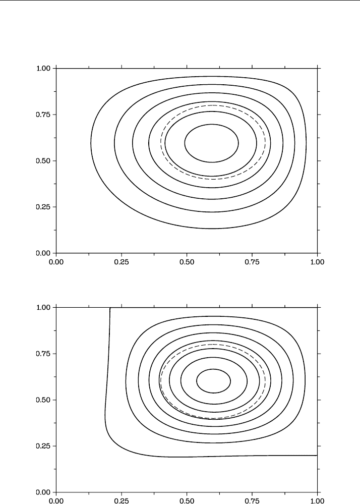
The end-time solution of the direct problem (the exact initial condition for the di-

rect problem) is shown in Figure 7.5. Here, contour lines obtained with u = 0.05 are

shown. Figure 7.6 shows the solution of the inverse problem obtained with δ = 0.01

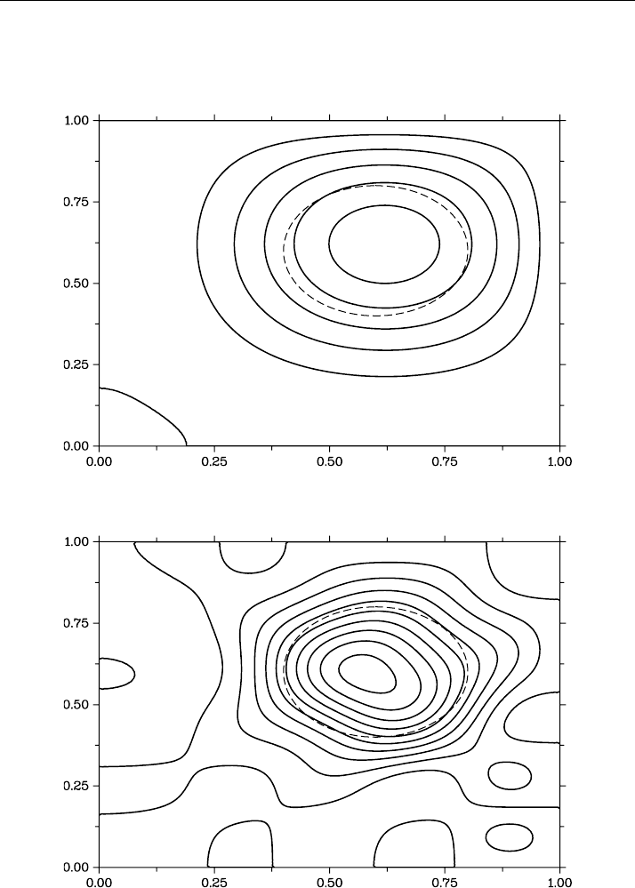
(here, u = 0.1). Since, in the present example, a discontinuous function is recon-

structed, one cannot expect that a very good accuracy can be achieved. The effect due

to the inaccuracy level can be traced considering Figures 7.7 and 7.8.

Section 7.2 Regularized difference schemes 289

Figure 7.5 Solution of the direct problem at t = T

Figure 7.6 Solution of the inverse problem obtained with δ = 0.01

290 Chapter 7 Evolutionary inverse problems

Figure 7.7 Solution of the inverse problem obtained with δ = 0.02

Figure 7.8 Solution of the inverse problem obtained with δ = 0.005

Section 7.3 Iterative solution of retrospective problems 291

7.3 Iterative solution of retrospective problems

Key features of algorithms intended for the approximate solution of inverted-time

problems by iteration methods with reﬁnement of initial conditions are outlined. A

model problem for the two-dimensional non-stationary parabolic equation is consid-

ered.

7.3.1 Statement of the problem

In solving inverse problems for mathematical physics equations, gradient iteration

methods are applied to the variational formulation of the problem. Below, we consider

a simplest iteration method for the approximate solution of the retrospective inverse

problem for the second-order parabolic equation. For this inverse problem, the ini-

tial condition is reﬁned iteratively, which requires solving, at each iteration step, an

ordinary boundary value problem for the parabolic equation.

Based on the general theory of iteration solution methods for operator equations,

sufﬁcient conditions for convergence of the iterative process can be established, and

the iteration parameters are chosen. In such problems, the operator of transition to the

next approximation makes it possible to identify the approximate solution in a desired

class of smoothness.

As a model problem, consider a two-dimensional problem in the rectangle

 ={x | x = (x

, x

), 0 < x

< l

,β= 1, 2}.

In the domain , we seek the solution of the parabolic equation

∂u

∂t

−



β=1

∂

∂x



k(x)

∂u

∂x



= 0, x ∈ , 0 < t < T , (7.159)

supplemented with the simplest ﬁrst-kind homogeneous boundary conditions:

u(x, t) = 0, x ∈ ∂, 0 < t < T . (7.160)

In the inverse problem, instead of setting the zero-time solution (the solution at t = 0),

the end-time solution is speciﬁed:

u(x, T ) = ϕ(x), x ∈ . (7.161)

Such an inverse problem is a well-posed one, for instance, in the classes of bounded

solutions.

292 Chapter 7 Evolutionary inverse problems

7.3.2 Difference problem

Performing discretization over space, we put into correspondence to the differential

problem (7.159)–(7.161) some differential-difference problem. For simplicity, we as-

sume that a grid uniform along either direction with steps h

, β = 1, 2 is introduced

in the domain , and let ω be the set of internal nodes.

On the set of mesh functions y(x) such that y(x) = 0, x ∈ ω, we deﬁne the

difference operator :

y =−



β=1

¯x

)

(7.162)

where, for instance,

(x) = k(x

− 0.5h

, x

), a

(x) = k(x

, x

− 0.5h

In the mesh Hilbert space H , we introduce the scalar product and the norm:

(y,w) =



x∈ω

y(x)w(x)h

, y=(y, y)

1/2

In H ,wehave = 

∗

> 0. We pass from (7.159)–(7.161) to the differential-operator

equation

+ y = 0, x ∈ ω, 0 < t < T (7.163)

with some given

y(T ) = ϕ, x ∈ ω. (7.164)

Previously, possible ways in constructing regularizing algorithms for the approxi-

mate solution of problem (7.163), (7.164) based on using perturbed equations or per-

turbed initial conditions were discussed. In this chapter, the inverse problem (7.163),

(7.164) will be solved by iteration methods.

7.3.3 Iterative reﬁnement of the initial condition

Here, we are going to employ methods in which, at each iteration step, the emerging

well-posed problems are solved using standard two-layer difference schemes.

Suppose that, instead of the inverse problem (7.163), (7.164), we treat the direct

problem for equation (7.163), in which, instead of (7.164), we use the initial condition

y(0) = v, x ∈ ω. (7.165)

We denote by y

the difference solution at the time t

= nτ , where τ>0 is the time

step size, so that N

τ = T . In the ordinary two-layer weighted scheme the passage to

Section 7.3 Iterative solution of retrospective problems 293

the next time layer in problem (7.163), (7.165) is to be made in accordance with

n+1

− y

+ (σ y

n+1

+ (1 − σ)y

) = 0,

n = 0, 1,...,N

− 1,

(7.166)

= v, x ∈ ω. (7.167)

As it is well known, the weighted scheme (7.166), (7.167) is absolutely stable if

σ ≥ 1/2, and there holds the following estimate of stability:

y

n+1

≤y

≤···≤y

=v,

n = 0, 1,...,N

− 1.

(7.168)

Thereby, the solution norm decreases with time.

To approximately solve the inverse problem (7.163), (7.164), we use a simplest

iterative process based on successive reﬁnement of the initial condition and on solving

at each iteration step the direct problem. Let us formulate the problem in the operator

form.

From (7.166) and (7.167), for the given y

at the end time we obtain

= S

v, (7.169)

where S is the operator of transition from one time layer to the next time layer:

S = (E + στ)

−1

(E + (σ − 1)τ ). (7.170)

In view of (7.163), (7.164), and (7.169), the approximate solution of the inverse

problem can be put into correspondence to the solution of the following difference

operator equation:

Av = ϕ, x ∈ ω, A = S

. (7.171)

Since the operator  is a self-adjoint operator, the transition operator S and the

operator A in (7.171) are also self-adjoint operators. The difference equation (7.171)

can be solved uniquely if, for instance, the operator A is a positive operator. In turn,

the latter condition is satisﬁed if the transition operator S is a positive operator. Taking

into account the representation (7.170), we obtain that S > 0 in the case of

σ ≥ 1. (7.172)

Condition (7.172) imposed on the weight of scheme (7.166), (7.167) is a more strin-

gent condition than the ordinary stability condition. In the case of interest, under the

constraints (7.172) for the operator A deﬁned by (7.171) we have:

0 < A = A

∗

< E. (7.173)

294 Chapter 7 Evolutionary inverse problems

Equation (7.171), (7.173) can be solved using the explicit two-layer iteration

method; this method can be written as

k+1

− v

k+1

+ Av

= ϕ. (7.174)

Here, s

k+1

are iteration parameters. We denote the difference solution obtained with

the initial condition v

as y

(k)

The iteration method under consideration implies the following organization of cal-

culations in the approximate solution of the retrospective inverse problem (7.159),

(7.160).

First, with the given v

, we solve the direct problem, using, for determining y

(k)

, the

difference scheme

(k)

n+1

− y

(k)

+ (σ y

(k)

n+1

+ (1 − σ)y

(k)

) = 0,

n = 0, 1,...,N

− 1,

(7.175)

(k)

= v

, x ∈ ω. (7.176)

Then, with the found end-time solution of the direct problem, we use formula

(7.174) to reﬁne the initial condition:

k+1

= v

− s

k+1

(k)

− ϕ). (7.177)

As it follows from the general theory of iterative solution methods, the rate of con-

vergence in method (7.174), used to solve equation (7.171), is deﬁned by the energy

equivalence constants γ

,β= 1, 2:

E ≤ A ≤ γ

E,γ

> 0. (7.178)

Regarding (7.173), we can put γ

= 1. The positive constant γ

, close to zero, depends

on the grid.

In the notation used, in the stationary iteration method (s

= s

= const) the condi-

tions for convergence in (7.174) have the form s

≤ 2. For the optimal constant value

of the iteration parameter we have: s

≈ 1. For the convergence to be improved, it

makes sense to use variation-type iteration methods. In the iteration method of mini-

mal discrepancies, for the iteration parameters we have:

k+1

(Ar

, r

)

(Ar

, Ar

)

, r

= Av

− ϕ.

Here, at each iteration step we minimize the discrepancy norm which implies the fol-

lowing estimate:

r

k+1

 < r

 < ···< r

.

Section 7.3 Iterative solution of retrospective problems 295

In the more general implicit iteration method, instead of (7.174) we have:

k+1

− v

k+1

+ Av

= ϕ, (7.179)

where B = B

∗

> 0. In the method of minimal corrections, iteration parameters can

be calculated by the formulas

k+1

(Aw

)

−1

, Aw

)

= B

−1

Here, to be minimized at each iteration step is the correction w

k+1

which implies the

estimate

w

k+1

 < w

 < ···< w

.

In a similar manner, more rapidly converging three-layer variational iteration methods

can be considered.

Note the following speciﬁc features in the choice of B in solving ill-posed problems.

In ordinary iteration methods the operator B is to be chosen so that just to raise the

rate of convergence in the method. In solving ill-posed problem, the iterative process

is to be terminated on attainment of a discrepancy value deﬁned by the input-data

inaccuracy. Of importance for us is not only the rate with which the iterative process

converges on the descending portion of the characteristic curve but also the class of

smoothness in which this iterative process converges and the norm with which the

required discrepancy level can be achieved. A key speciﬁc feature of the approximate

solution of ill-posed problems by iteration methods consists in that the approximate

solution can be identiﬁed in the desired class of smoothness using a proper choice

of B.

7.3.4 Program

The iteration method under consideration is based on reﬁnement of the initial condition

for the solution of a well-examined direct problem. For the implicit difference schemes

(7.175), (7.176) to be realized, we have to solve at each time step two-dimensional

difference elliptic problems. To this end, we use iteration methods (embedded iterative

process).

Program PROBLEM12

C PROBLEM12 - PROBLEM WITH INVERTED TIME

C TWO-DIMENSIONAL PROBLEM

C ITERATIVE REFINEMENT OF THE INITIAL CONDITION

IMPLICIT REAL

8 ( A-H, O-Z )

PARAMETER ( DELTA = 0.01D0, N1 = 51, N2 = 51, M = 101 )

DIMENSION A(17

N2), X1(N1), X2(N2)

COMMON / SB5 / IDEFAULT(4)