Samarskii A.A., Vabishchevich P.N. Numerical Methods for Solving Inverse Problems of Mathematical Physics

Подождите немного. Документ загружается.

296 Chapter 7 Evolutionary inverse problems

COMMON / CONTROL / IREPT, NITER

C PARAMETERS:

C X1L, X2L - COORDINATES OF THE LEFT CORNER;

C X1R, X2R - COORDINATES OF THE RIGHT CIRNER;

C N1, N2 - NUMBER OF NODES IN THE SPATIAL GRID;

C H1, H2 - MESH SIZES OVER SPACE;

C TAU - TIME STEP;

C DELTA - INPUT-DATA INACCURACY LEVEL;

C U0(N1,N2) - INITIAL CONDITION TO BE RECONSTRUCTED;

C UT(N1,N2) - END-TIME SOLUTION IN THE DIRECT PROBLEM;

C UTD(N1,N2)- DISTURBED DIRECT-PROBLEM SOLUTION;

C U(N1,N2) - APPROXIMATE SOLUTION IN THE INVERSE PROBLEM;

C EPSR - RELATIVE INACCURACY OF THE DIFFERENCE SOLUTION;

C EPSA - ABSOLUTE INACCURACY OF THE DIFFERENCE SOLUTION;

C EQUIVALENCE ( A(1), A0 ),

( A(N+1), A1 ),

( A(2

N+1), A2 ),

( A(9

N+1), F ),

( A(10

N+1), U0 ),

( A(11

N+1), UT ),

( A(12

N+1), UTD ),

( A(13

N+1), U ),

( A(14

N+1), V ),

( A(15

N+1), R ),

( A(16

N+1), BW )

X1L = 0.D0

X1R = 1.D0

X2L = 0.D0

X2R = 1.D0

TMAX = 0.025D0

PI = 3.1415926D0

EPSR = 1.D-5

EPSA = 1.D-8

OPEN (01, FILE =’RESULT.DAT’) ! FILE TO STORE THE CALCULATED DATA

C GRID

H1 = (X1R-X1L) / (N1-1)

H2 = (X2R-X2L) / (N2-1)

TAU = TMAX / (M-1)

DOI=1,N1

X1(I) = X1L + (I-1)

END DO

DOJ=1,N2

X2(J) = X2L + (J-1)

END DO

N=N1

DOI=1,17

A(I) = 0.0

END DO

C DIRECT PROBLEM

C PURELY IMPLICIT DIFFERENCE SCHEME

Section 7.3 Iterative solution of retrospective problems 297

C INITIAL CONDITION

T = 0.D0

CALL INIT (A(10

N+1), X1, X2, N1, N2)

DOK=2,M

C DIFFERENCE-SCHEME COEFFICIENTS IN THE DIRECT PROBLEM

CALL FDST (A(1), A(N+1), A(2

N+1), A(9

N+1), A(10

N+1),

+ H1, H2, N1, N2, TAU)

C SOLUTION OF THE DIFFERENCE PROBLEM

IDEFAULT(1) = 0

IREPT = 0

CALL SBAND5 (N, N1, A(1), A(10

N+1), A(9

N+1), EPSR, EPSA)

END DO

C DISTURBING OF MEASURED QUANTITIES

DOI=1,N

A(11

N+I) = A(10

N+I)

A(12

N+I) = A(11

N+I) + 2.

DELTA

(RAND(0)-0.5)

END DO

C INVERSE PROBLEM

C ITERATION METHOD

IT=0

C STARTING APPROXIMATION

DOI=1,N

A(14

N+I) = 0.D0

END DO

100IT=IT+1

C DIRECT PROBLEM

T = 0.D0

C INITIAL CONDITION

DOI=1,N

A(10

N+I) = A(14

N+I)

END DO

DOK=2,M

C DIFFERENCE-SCHEME COEFFICIENTS IN THE DIRECT PROBLEM

CALL FDST (A(1), A(N+1), A(2

N+1), A(9

N+1), A(10

N+1),

+ H1, H2, N1, N2, TAU)

C SOLUTION OF THE DIFFERENCE PROBLEM

IDEFAULT(1) = 0

IREPT = 0

CALL SBAND5 (N, N1, A(1), A(10

N+1), A(9

N+1), EPSR, EPSA)

298 Chapter 7 Evolutionary inverse problems

END DO

C DISCREPANCY

DOI=1,N

A(15

N+I) = A(10

N+I) - A(12

N+I)

END DO

C CORRECTION

C DIFFERENCE-SCHEME COEFFICIENTS IN THE DIRECT PROBLEM

CALL FDSB (A(1), A(N+1), A(2

N+1), A(9

N+1), A(15

N+1),

+ H1, H2, N1, N2)

C SOLUTION OF THE DIFFERENCE PROBLEM

IDEFAULT(1) = 0

IREPT = 0

CALL SBAND5 (N, N1, A(1), A(13

N+1), A(9

N+1), EPSR, EPSA)

C ITERATION PARAMETERS

T = 0.D0

C INITIAL CONDITIONS

DOI=1,N

A(10

N+I) = A(13

N+I)

END DO

DOK=2,M

C DIFFERENCE-SCHEME COEFFICIENTS IN THE DIRECT PROBLEM

CALL FDST (A(1), A(N+1), A(2

N+1), A(9

N+1), A(10

N+1),

+ H1, H2, N1, N2, TAU)

C SOLUTION OF THE DIFFERENCE PROBLEM

IDEFAULT(1) = 0

IREPT = 0

CALL SBAND5 (N, N1, A(1), A(10

N+1), A(9

N+1), EPSR, EPSA)

END DO

C METHOD OF MINIMAL DISCREPANCIES

C DIFFERENCE-SCHEME COEFFICIENTS IN THE DIRECT PROBLEM

CALL FDSB (A(1), A(N+1), A(2

N+1), A(9

N+1), A(10

N+1),

+ H1, H2, N1, N2)

C SOLUTION OF THE DIFFERENCE PROBLEM

IDEFAULT(1) = 0

IREPT = 0

CALL SBAND5 (N, N1, A(1), A(16

N+1), A(9

N+1), EPSR, EPSA)

SUM = 0.D0

SUM1 = 0.D0

DOI=1,N

Section 7.3 Iterative solution of retrospective problems 299

SUM = SUM + A(10

N+I)

A(13

N+I)

SUM1 = SUM1 + A(16

N+I)

A(10

N+I)

END DO

SS = SUM / SUM1

C NEXT APPROXIMATION

DOI=1,N

A(14

N+I) = A(14

N+I) - SS

A(13

N+I)

END DO

C EXIT FROM THE ITERATIVE PROCESS BY THE DISCREPANCY CRITERION

SUM = 0.D0

DOI=1,N

SUM = SUM + A(15

N+I)

END DO

SL2 = DSQRT(SUM)

IF ( SL2.GT.DELTA ) GO TO 100

C SOLUTION

DOI=1,N

A(13

N+I) = A(14

N+I)

END DO

WRITE ( 01,

) (A(11

N+I), I=1,N)

WRITE ( 01,

) (A(13

N+I), I=1,N)

CLOSE (01)

STOP

END

SUBROUTINE INIT (U, X1, X2, N1, N2)

C INITIAL CONDITION

IMPLICIT REAL

8 ( A-H, O-Z )

DIMENSION U(N1,N2), X1(N1), X2(N2)

DOI=1,N1

DOJ=1,N2

U(I,J) = 0.D0

IF ((X1(I)-0.6D0)

2 + (X2(J)-0.6D0)

2.LE.0.04D0)

+ U(I,J) = 1.D0

END DO

RETURN

END

SUBROUTINE FDST (A0, A1, A2, F, U, H1, H2, N1, N2, TAU)

C GENERATION OF DIFFERENCE-SCHEME COEFFICIENTS

C FOR THE PARABOLIC EQUATION WITH CONSTANT COEFFICIENTS

C IN THE CASE OF PURELY IMPLICIT SCHEME

IMPLICIT REAL

8 ( A-H, O-Z )

DIMENSION A0(N1,N2), A1(N1,N2), A2(N1,N2), F(N1,N2), U(N1,N2)

DOJ=2,N2-1

DOI=2,N1-1

A1(I-1,J) = 1.D0/(H1

H1)

300 Chapter 7 Evolutionary inverse problems

A1(I,J) = 1.D0/(H1

H1)

A2(I,J-1) = 1.D0/(H2

H2)

A2(I,J) = 1.D0/(H2

H2)

A0(I,J) = A1(I,J) + A1(I-1,J) + A2(I,J) + A2(I,J-1)

+ + 1.D0/TAU

F(I,J) = U(I,J)/TAU

END DO

C FIRST-KIND HOMOGENEOUS BOUNDARY CONDITION

DOJ=2,N2-1

A0(1,J) = 1.D0

A1(1,J) = 0.D0

A2(1,J) = 0.D0

F(1,J) = 0.D0

END DO

DOJ=2,N2-1

A0(N1,J) = 1.D0

A1(N1-1,J) = 0.D0

A1(N1,J) = 0.D0

A2(N1,J) = 0.D0

F(N1,J) = 0.D0

END DO

DOI=2,N1-1

A0(I,1) = 1.D0

A1(I,1) = 0.D0

A2(I,1) = 0.D0

F(I,1) = 0.D0

END DO

DOI=2,N1-1

A0(I,N2) = 1.D0

A1(I,N2) = 0.D0

A2(I,N2) = 0.D0

A2(I,N2-1) = 0.D0

F(I,N2) = 0.D0

END DO

A0(1,1) = 1.D0

A1(1,1) = 0.D0

A2(1,1) = 0.D0

F(1,1) = 0.D0

A0(N1,1) = 1.D0

A2(N1,1) = 0.D0

F(N1,1) = 0.D0

A0(1,N2) = 1.D0

A1(1,N2) = 0.D0

F(1,N2) = 0.D0

A0(N1,N2) = 1.D0

F(N1,N2) = 0.D0

RETURN

END

Section 7.3 Iterative solution of retrospective problems 301

SUBROUTINE FDSB (A0, A1, A2, F, U, H1, H2, N1, N2)

C GENERATION OF DIFFERENCE-SCHEME COEFFICIENTS

C FOR THE DIFFERENCE ELLIPTIC EQUATION

IMPLICIT REAL

8 ( A-H, O-Z )

DIMENSION A0(N1,N2), A1(N1,N2), A2(N1,N2), F(N1,N2), U(N1,N2)

DOJ=2,N2-1

DOI=2,N1-1

A1(I-1,J) = 1.D0/(H1

H1)

A1(I,J) = 1.D0/(H1

H1)

A2(I,J-1) = 1.D0/(H2

H2)

A2(I,J) = 1.D0/(H2

H2)

A0(I,J) = A1(I,J) + A1(I-1,J) + A2(I,J) + A2(I,J-1)

+ + 1.D0

F(I,J) = U(I,J)

END DO

C FIRST-KIND HOMOGENEOUS BOUNDARY CONDITIONS

DOJ=2,N2-1

A0(1,J) = 1.D0

A1(1,J) = 0.D0

A2(1,J) = 0.D0

F(1,J) = 0.D0

END DO

DOJ=2,N2-1

A0(N1,J) = 1.D0

A1(N1-1,J) = 0.D0

A1(N1,J) = 0.D0

A2(N1,J) = 0.D0

F(N1,J) = 0.D0

END DO

DOI=2,N1-1

A0(I,1) = 1.D0

A1(I,1) = 0.D0

A2(I,1) = 0.D0

F(I,1) = 0.D0

END DO

DOI=2,N1-1

A0(I,N2) = 1.D0

A1(I,N2) = 0.D0

A2(I,N2) = 0.D0

A2(I,N2-1) = 0.D0

F(I,N2) = 0.D0

END DO

A0(1,1) = 1.D0

A1(1,1) = 0.D0

A2(1,1) = 0.D0

F(1,1) = 0.D0

A0(N1,1) = 1.D0

A2(N1,1) = 0.D0

F(N1,1) = 0.D0

302 Chapter 7 Evolutionary inverse problems

A0(1,N2) = 1.D0

A1(1,N2) = 0.D0

F(1,N2) = 0.D0

A0(N1,N2) = 1.D0

F(N1,N2) = 0.D0

RETURN

END

In the subroutine FDST, coefﬁcients of the difference elliptic problem are generated

for the problem to be solved at the next time step. In the subroutine FDSB, coefﬁcients

of the difference elliptic operator B in the iterative process (7.179) are generated, so

that

By =−



β=1

¯x

+ y.

Difference elliptic problems are solved in the subroutine SBAND5.

7.3.5 Computational experiments

Like in the case of regularized difference schemes intended for approximate solution

of inverted-time problems, a uniform grid with h

= 0.02 and h

= 0.02 for the

model problem with k(x) = 1 in unit square was used. In the framework of a quasi-

real experiment, the direct problem with T = 0.025 is solved using a time grid with

τ = 0.00025. A purely implicit difference scheme (σ = 1) was employed. Again,

in the direct problem the initial condition (the exact end-time solution of the inverse

problem) is given by

(x, 0) =



1,(x

− 0.6)

+ (x

− 0.6)

≤ 0.04,

0,(x

− 0.6)

+ (x

− 0.6)

> 0.04.

The end-time solution of the direct problem is shown in Figure 7.5.

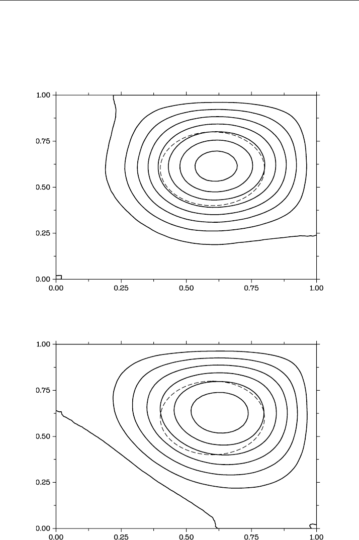
To illustrate the capability of the adopted scheme in reconstructing a piecewise-

discontinuous initial condition, here we present computational data obtained with un-

perturbed input data (the difference solution of the direct problem at t = T ). The

iterative process was terminated when the difference r

= Av

− ϕ attained the es-

timate r

≤ε. Approximate solutions obtained with ε = 0.001 and ε = 0.0001

are shown in Figures 7.9 and 7.10, respectively (in the ﬁgures, contour lines with the

step size u = 0.05 are plotted). A substantial (tenfold) change in the solution accu-

racy for the inverse problem results in slight reﬁnement of the approximate solution.

In the case of interest, we cannot expect that a more accurate reconstruction of the

piecewise-discontinuous initial condition can be achieved.

Section 7.3 Iterative solution of retrospective problems 303

Figure 7.9 Inverse-problem solution obtained with ε = 0.001

Figure 7.10 Inverse-problem solution obtained with ε = 0.0001

304 Chapter 7 Evolutionary inverse problems

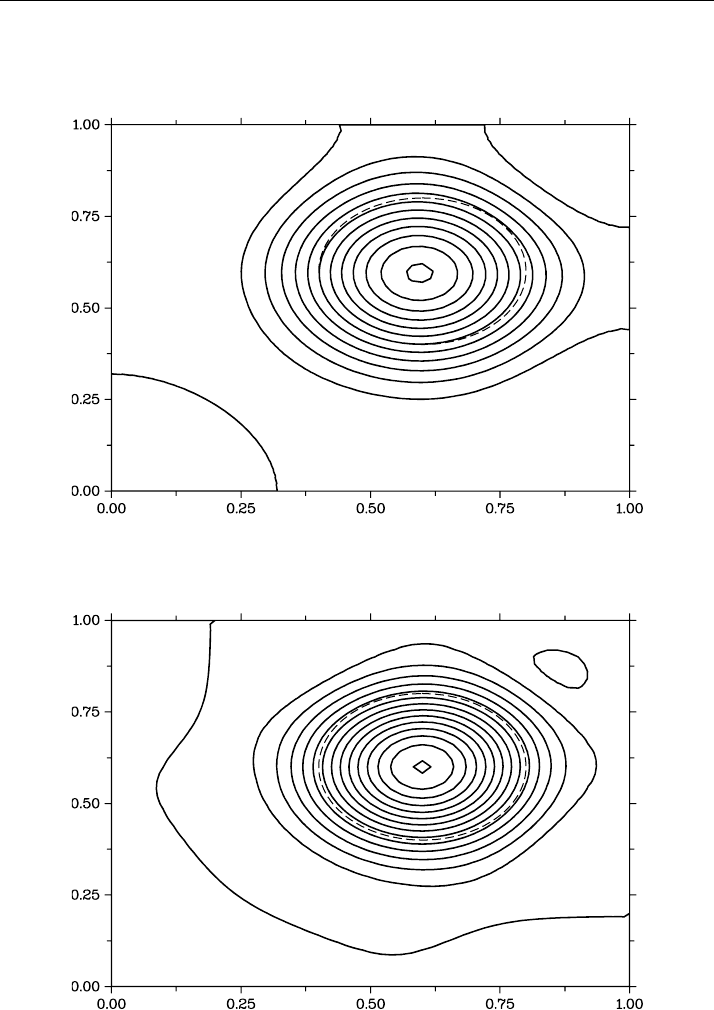
In perturbing input data, we have to try identify the smooth initial solution of the

inverse problem using a proper choice of the operator B = E in the iterative pro-

cess (7.179). Figure 7.11 shows the solution of the inverse problem obtained at the

inaccuracy level δ = 0.01. Solutions of the problem obtained at a higher and lower

inaccuracy levels are shown in Figures 7.12 and 7.13.

Figure 7.11 Inverse-problem solution obtained with δ = 0.01

Figure 7.12 Inverse-problem solution obtained with δ = 0.02

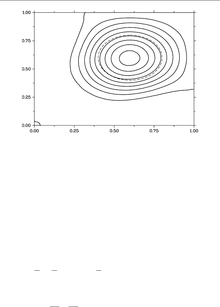
Section 7.4 Second-order evolution equation 305

Figure 7.13 Inverse-problem solution obtained with δ = 0.005

7.4 Second-order evolution equation

A classical example of ill-posed problems is the Cauchy problem for the elliptic equa-

tion (Hadamard examples). In this section, major possibilities available in the con-

struction of stable solution algorithm for such evolutionary inverse problems are con-

sidered. Methods using the perturbation of initial conditions and the perturbation of

the initial second-order evolution equation are brieﬂy discussed. A program in which,

to approximately solve the Cauchy problem for the Laplace equation, regularized dif-

ference schemes are used, is presented.

7.4.1 Model problem

Consider the simplest inverse problem for the two-dimensional Laplace equation. Let

us start with formulating the direct problem. Suppose that in the rectangle

=  × [0, T ],  ={x | 0 ≤ x ≤ l}, 0 ≤ t ≤ T

the function u(x, t) satisﬁes the equation

∂

∂t

∂

∂x

= 0, 0 < x < l, 0 < t < T. (7.180)

We supplement this equation with some boundary conditions. On the lateral sides of

the rectangle, we put:

u(0, t) = 0, u(l, t) = 0, 0 < t < T. (7.181)