Samarskii A.A., Vabishchevich P.N. Numerical Methods for Solving Inverse Problems of Mathematical Physics

Подождите немного. Документ загружается.

316 Chapter 7 Evolutionary inverse problems

Scheme (7.240) can be written in the canonical form for three-layer difference

schemes

n+1

− y

n−1

2τ

+ R(y

n+1

− 2y

+ y

n−1

) + Ay

= 0 (7.241)

with operators

B = 0, R =

E, A =−, (7.242)

i. e., with A = A

∗

< 0.

Theorem 7.24 The explicit scheme (7.240) is ρ-stable with

ρ = exp (M

1/2

τ). (7.243)

Proof. For scheme (7.240), we check that the following conditions for ρ-stability (see

Theorem 4.11) are fulﬁlled:

+ 1

B + τ(ρ

− 1)R ≥ 0, (7.244)

− 1

2τ

B + (ρ − 1)

R + ρ A > 0, (7.245)

− 1

2τ

B + (ρ + 1)

R − ρ A > 0. (7.246)

Apparently, in the case of B ≥ 0, A ≤ 0, R ≥ 0 and ρ>1 (see (7.242)) inequalities

(7.244) and (7.246) are fulﬁlled for all τ>0.

With (7.242), inequality (7.245) yields:

(ρ − 1)

E − τ

ρ ≥ ((ρ − 1)

−1

− τ

ρ) > 0.

Derivation of the estimates is based on the following useful result.

Lemma 7.25 Inequality

(ρ − 1)

χ −τ

ρ>0 (7.247)

is fulﬁlled for positive χ , τ and for ρ>1 in the case of

ρ ≥ exp



−1/2



Proof. Inequality (7.247) is fulﬁlled in the case of ρ>ρ

, where

= 1 +

−1

+ τχ

−1/2



1 +

−1



1/2

Taking into account the inequality



1 +

−1



1/2

< 1 +

−1

Section 7.4 Second-order evolution equation 317

we obtain

< 1 + τχ

−1/2

−1

−3/2

< 1 + τχ

−1/2

−1

−3/2

< exp (χ

−1/2

τ).

Thus, the lemma is proved.

In the case of interest, we have χ = M

−1

and, hence, for ρ we obtain the desired

estimate (4.32) for the explicit scheme (7.240).

With regard to the boundedness of  (in Cauchy problems for elliptic equations),

we conclude that the grid step over space limits the solution growth, i.e., serves the

regularization parameter.

Let us construct now, at the expense of introducing penalty terms into the difference

operators of difference schemes, unconditionally stable difference schemes for the ap-

proximate solution of problem (7.237)–(7.239). Starting from the explicit scheme

(7.240), we write the regularized scheme in the canonical form (7.241) with

B = 0, R =

(E + αG), A =−. (7.248)

Theorem 7.26 The regularized scheme (7.241), (7.248) is ρ-stable with the regulizer

G =  with

ρ = exp



√



, (7.249)

and with the regulizer G = 

, with

ρ = exp





√



. (7.250)

Proof. Starting from (7.245) for (7.248), we arrive at the inequality

(ρ − 1)

(E + αG) − τ

ρ ≥ 0. (7.251)

In the case of G = , analogously to the proof of Theorem 7.24 (χ = α + M

−1

)

we obtain the following expression for ρ:

ρ = exp



(α +

−1

)

−1/2



Making ρ cruder yields the estimate (7.249).

In the case of G = 

, from inequality (7.245) we obtain:

E +α

−

(ρ − 1)

 =



√

α −

√

α(ρ − 1)





1 −

4α(ρ − 1)



318 Chapter 7 Evolutionary inverse problems

This inequality is fulﬁlled for some given ρ if

α ≥

4(ρ − 1)

. (7.252)

Let us evaluate now the quantity ρ for given α from inequality (7.252) rewritten in the

form

(ρ − 1)

√

α − τ

ρ.

By the above lemma with χ = 2

√

α, the latter inequality is fulﬁlled for the values of ρ

deﬁned by (7.250).

The regularized scheme (7.241), (7.248) with the regularizer G =  can be written

as the weighted scheme

n+1

− 2y

+ y

n−1

− (σ y

n+1

+ (1 − 2σ)y

+ σ y

n−1

) = 0 (7.253)

with σ =−α/τ

. Thereby, the regularizing parameter here is the negative weight in

(7.253). The latter scheme can also be related to a version of the generalized inverse

method (7.225) for the approximate solution of the ill-posed problem (7.187)–(7.189).

The construction of the regularized difference scheme is based on a perturbation

of the operators in the generic difference scheme (7.241), (7.242) chosen so that to

fulﬁll the operator inequality (7.245). In Theorem 7.26, the latter can be achieved

at the expense of some additive perturbation (increase) of R. There are many other

possibilities. In particular, note the possibility of additive perturbation of B:

B = αG, R =

E, A =−. (7.254)

Theorem 7.27 The regularized scheme (7.241), (7.254) with G =  is ρ-stable with

ρ = exp





. (7.255)

Proof. Inequality (7.245) can be rearranged as

− 1

2τ

B + (ρ − 1)

R + ρ A >

− 1

2τ

α −ρ ≥ 0.

This inequality is fulﬁlled with ρ ≥ ρ

, where



1 +



1/2

< 1 +

< exp





From here, expression (7.255) for ρ in the difference scheme (7.241), (7.254) follows.

The regularized scheme (7.241), (7.254) can be directly related to the use of the gen-

eralized inverse method in its version (7.234). In a similar way, regularized schemes

can be constructed which can be related to the basic variant (7.225) of the generalized

inverse method.

Section 7.4 Second-order evolution equation 319

7.4.6 Program

Here, we do not has as our object to check the efﬁciency of all mentioned methods for

the approximate solution of the model Cauchy problem for elliptic equation (7.180)–

(7.182), (7.184). As judged from the standpoint of computational realization, the sim-

plest approach here is related with using regularized schemes of type (7.241), (7.248)

(or (7.241), (7.254)) with the regulizer G = .

In the case of (7.241), (7.248), the approximate solution is to be found from the

difference equation

(E + α)

n+1

− 2y

+ y

n−1

− y

= 0,

and in the case of (7.241), (7.254), from

α

n+1

− y

n−1

2τ

n+1

− 2y

+ y

n−1

− y

= 0.

For such schemes, the computational realization is not much more difﬁcult than for

direct problems.

Here, to be controlled (bounded) is the growth of the solution norm, this very often

being not sufﬁcient for obtaining a satisfactory approximate solution. The latter cir-

cumstance is related with the fact that, here, we do not use any preliminary treatment

of the approximate solution burdened with input-data inaccuracy. That is why we have

to use regularized difference schemes with stronger regulizers.

The program PROBLEM13 realizes the regularized difference scheme (7.241),

(7.248) with G = 

(E + α

)

n+1

− 2y

+ y

n−1

− y

= 0. (7.256)

For the model problem (7.180)–(7.182), (7.184), the realization of (7.256) is based on

using the ﬁve-point sweep algorithm.

Note some possibilities available in choosing the regularization parameter. In the

most natural approach, the regularization parameter is to be chosen considering the

discrepancy; here, we compare, at t = 0, the solutions of the direct problem of type

(7.180)–(7.183), in which the boundary condition (7.183) is formulated from the solu-

tion of the inverse problem. Here, two circumstances are to be mentioned, which make

this approach very natural as used with regularized difference schemes of type (7.256).

First, the used algorithm becomes a global regularization algorithm (we have to solve

the problem for all times t at ones). Second, here the computational realization of

the direct problem, i.e., the boundary value problem for the elliptic equation, is much

more difﬁcult than for the inverse problem, a problem for the second-order evolution

equation.

320 Chapter 7 Evolutionary inverse problems

With the aforesaid, for choosing the value of the regularization parameter we have

to apply such algorithms that retain the local regularization property (making a con-

secutive determination of the approximate solution at the next time layer possible). A

simplest such algorithm is realized in the program PROBLEM13.

Previously (see (7.140)–(7.143)), the relation between the regularized schemes and

the difference-smoothing algorithms was elucidated. We rewrite scheme (7.256) as

˜w

− y

= 0,

(E + α

=˜w

n+1

where

n+1

− 2y

+ y

n−1

In this way, the second difference derivative is ﬁrst to be calculated by an explicit

formula and, then, to be smoothed:

) = min

v∈H

(v),

(v) =v −˜w



+ αv

In the case under consideration, the regularization is related with smoothing of mesh

functions.

First of all, the smoothing procedure has to be applied to the inaccurate input data.

Here, these data are the mesh function y

. In accordance with the discrepancy princi-

ple, the regularization (smoothing) parameter can be found from the condition

y

− u

=δ,

with

) = min

v∈H

(v),

(v) =v − u



+ αv

Program PROBLEM13

C PROBLEM13 - CAUCHY PROBLEM FOR THE LAPLACE EQUATION

C TWO-DIMENSIONAL PROBLEM

C REGULARIZED SCHEME

IMPLICIT REAL

8 ( A-H, O-Z )

PARAMETER ( DELTA = 0.005D0,N=65,M=65)

DIMENSION U0(N), U0D(N), UT(N), U(N), U1(N), Y(N), Y1(N)

+ ,X(N), A(N), B(N), C(N), D(N), E(N), F(N)

C PARAMETERS:

Section 7.4 Second-order evolution equation 321

C XL, XR - LEFT AND RIGHT ENDS OF THE SEGMENT;

C N - NUMBER OF NODES IN THE SPATIAL GRID;

C TMAX - MAXIMAL TIME;

C M - NUMBER OF NODES OVER TIME;

C DELTA - INPUT-DATA INACCURACY LEVEL;

C Q - FACTOR IN THE FORMULA FOR THE REGULARIZATION PARAMETER;

C U0(N) - INITIAL CONDITION;

C U0D(N) - DISTURBED INITIAL CONDITION;

C UT(N) - EXACT END-TIME SOLUTION;

C U(N) - APPROXIMATE SOLUTION OF THE INVERSE PROBLEM;

XL = 0.D0

XR = 1.D0

TMAX = 0.25D0

OPEN (01, FILE = ’RESULT.DAT’)! FILE TO STORE THE CALCULATED DATA

C GRID

H=(XR-XL)/(N-1)

TAU = TMAX / (M-1)

DOI=1,N

X(I) = XL + (I-1)

END DO

C EXACT SOLUTION OF THE PROBLEM

DOI=1,N

U0(I) = AU(X(I), 0.D0)

UT(I) = AU(X(I), TMAX)

END DO

C DISTURBING OF MEASURED QUANTITIES

DOI=2,N-1

U0D(I) = U0(I) + 2.

DELTA

(RAND(0)-0.5)

END DO

U0D(1) = U0(1)

U0D(N) = U0(N)

C INVERSE PROBLEM

C SMOOTHING OF INITIAL CONDITIONS

IT=0

ITMAX = 100

ALPHA = 0.00001D0

Q = 0.75D0

100IT=IT+1

C DIFFERENCE-SCHEME COEFFICIENTS IN THE INVERSE PROBLEM

DOI=2,N-1

A(I) = ALPHA / (H

B(I) = 4.D0

ALPHA / (H

C(I) = 6.D0

ALPHA / (H

4) + 1.D0

D(I) = 4.D0

ALPHA / (H

E(I) = ALPHA / (H

END DO

C(1) = 1.D0

322 Chapter 7 Evolutionary inverse problems

D(1) = 0.D0

E(1) = 0.D0

F(1) = 0.D0

B(2) = 0.D0

C(2) = 5.D0

ALPHA / (H

4) + 1.D0

C(N-1) = 5.D0

ALPHA / (H

4) + 1.D0

D(N-1) = 0.D0

A(N) = 0.D0

B(N) = 0.D0

C(N) = 1.D0

F(N) = 0.D0

DOI=2,N-1

F(I) = U0D(I)

END DO

C SOLUTION OF THE DIFFERENCE PROBLEM

ITASK = 1

CALL PROG5 ( N, A, B, C, D, E, F, U1, ITASK )

C CRITERION FOR THE EXIT FROM THE ITERATIVE PROCESS

WRITE (01,

) IT, ALPHA

SUM = 0.D0

DOI=2,N-1

SUM = SUM + (U1(I) - U0D(I))

END DO

SL2 = DSQRT(SUM)

IF (IT.GT.ITMAX) STOP

IF ( IT.EQ.1 ) THEN

IND=0

IF ( SL2.LT.DELTA ) THEN

IND=1

Q = 1.D0/Q

END IF

ALPHA = ALPHA

GO TO 100

ELSE

ALPHA = ALPHA

IF ( IND.EQ.0 .AND. SL2.GT.DELTA ) GO TO 100

IF ( IND.EQ.1 .AND. SL2.LT.DELTA ) GO TO 100

END IF

C INVERSE-PROBLEM SOLUTION WITH CHOSEN REGULARIZATION PARAMETER

C REGULARIZED SCHEME

C INITIAL CONDITION

DOI=1,N

Y1(I) = U1(I)

END DO

DOI=2,N-1

Y(I) = Y1(I)

+ + 0.5D0

TAU

2/H

(Y1(I+1)-2.D0

Y1(I) + Y1(I-1))

END DO

Y(1) = 0.D0

Y(N) = 0.D0

DOK=3,M

Section 7.4 Second-order evolution equation 323

C DIFFERENCE-SCHEME COEFFICIENTS IN THE INVERSE PROBLEM

DOI=2,N-1

A(I) = ALPHA / (H

B(I) = 4.D0

ALPHA / (H

C(I) = 6.D0

ALPHA / (H

4) + 1.D0

D(I) = 4.D0

ALPHA / (H

E(I) = ALPHA / (H

END DO

C(1) = 1.D0

D(1) = 0.D0

E(1) = 0.D0

F(1) = 0.D0

B(2) = 0.D0

C(2) = 5.D0

ALPHA / (H

4) + 1.D0

C(N-1) = 5.D0

ALPHA / (H

4) + 1.D0

D(N-1) = 0.D0

A(N) = 0.D0

B(N) = 0.D0

C(N) = 1.D0

F(N) = 0.D0

DOI=3,N-2

F(I) = A(I)

(2.D0

Y(I-2) - Y1(I-2))

+ - B(I)

(2.D0

Y(I-1) - Y1(I-1))

+ + C(I)

(2.D0

Y(I) - Y1(I))

+ - D(I)

(2.D0

Y(I+1) - Y1(I+1))

+ + E(I)

(2.D0

Y(I+2) - Y1(I+2))

+ - TAU

2/(H

(Y(I+1)-2.D0

Y(I) + Y(I-1))

END DO

F(2) = - B(2)

(2.D0

Y(1) - Y1(1))

+ + C(2)

(2.D0

Y(2) - Y1(2))

+ - D(2)

(2.D0

Y(3) - Y1(3))

+ + E(2)

(2.D0

Y(4) - Y1(4))

+ - TAU

2/(H

(Y(3)-2.D0

Y(2) + Y(1))

F(N-1) = A(N-1)

(2.D0

Y(N-3) - Y1(N-3))

+ - B(N-1)

(2.D0

Y(N-2) - Y1(N-2))

+ + C(N-1)

(2.D0

Y(N-1) - Y1(N-1))

+ - D(N-1)

(2.D0

Y(N) - Y1(N))

+ - TAU

2/(H

(Y(N)-2.D0

Y(N-1) + Y(N-2))

C SOLUTION OF THE DIFFERENCE PROBLEM

DOI=1,N

Y1(I) = Y(I)

END DO

ITASK = 1

CALL PROG5 ( N, A, B, C, D, E, F, Y, ITASK )

END DO

DOI=1,N

U(I) = Y(I)

END DO

C SOLUTION

WRITE ( 01,

) (U0(I),I=1,N)

WRITE ( 01,

) (UT(I),I=1,N)

WRITE ( 01,

) (U0D(I),I=1,N)

WRITE ( 01,

) (X(I),I=1,N)

WRITE ( 01,

) (U(I),I=1,N)

324 Chapter 7 Evolutionary inverse problems

CLOSE (01)

STOP

END

DOUBLE PRECISION FUNCTION AU ( X, T )

IMPLICIT REAL

8 ( A-H, O-Z )

C EXACT SOLUTION

PI = 3.1415926D0

C1 = 0.1D0

C2 = 0.5D0

AU=C1

(DEXP(PI

T) + DEXP(-PI

T))

DSIN(PI

++C2

(DEXP(2

T) + DEXP(-2

T))

DSIN(2

RETURN

END

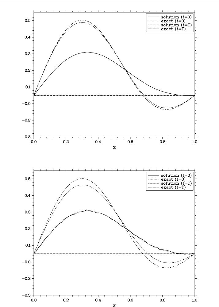
7.4.7 Computational experiments

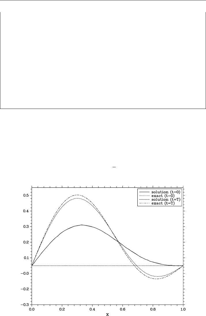
The data presented below were obtained on a uniform grid with h = 1/64 and l = 1.

The inverse problem was solved till the time T = 0.25, the time step size of the grid

being τ = T/64. The exact solution of the inverse problem is

u(x, t) = ch (πt) sin (πx) +

ch (2π t) sin (2π x).

Figure 7.14 Solution of the problem obtained with δ = 0.002

Section 7.4 Second-order evolution equation 325

Figure 7.15 Solution of the problem obtained with δ = 0.001

Figure 7.16 Inverse-problem solution obtained with δ = 0.005

Figure 7.14 shows the solution of the inverse problem obtained for the inaccuracy

level deﬁned by the quantity δ = 0.002. Here, the exact and perturbed initial condi-