Samarskii A.A., Vabishchevich P.N. Numerical Methods for Solving Inverse Problems of Mathematical Physics

Подождите немного. Документ загружается.

326 Chapter 7 Evolutionary inverse problems

tions are shown, as well as the exact and approximate end-time solution of the inverse

problem. Solutions of the problem obtained for two other inaccuracy levels are shown

in Figures 7.15 and 7.16. The calculation data prove it possible to reconstruct smooth

solutions at inaccuracy levels amounting to one percent.

7.5 Continuation of non-stationary ﬁelds

from point observation data

In this section, we consider the inverse problem for a model non-stationary parabolic

equation with unknown initial condition and with information about the solution avail-

able at some points of the two-dimensional calculation domain. We describe a com-

putational algorithm developed around the variational formulation of the problem and

using the Tikhonov regularization algorithm.

7.5.1 Statement of the problem

We consider a problem in which it is required to determine a non-stationary ﬁeld

u(x, t) that satisﬁes a second-order parabolic equation in a bounded two-dimensional

domain  and certain boundary conditions provided that information about the solu-

tion at some points in the domain is available. The initial state u(x, 0) is assumed

unknown. This problem is an ill-posed one; in particular, we cannot rely on obtaining

a unique solution. Such inverse problems often arise in hydrogeology, for instance, in

the cases in which all available information about the solution is given by variation of

physical quantities in observation holes.

In a two-dimensional bounded domain  (x = (x

, x

)), we seek the solution of the

parabolic equation

∂u

∂t

−



β=1

∂

∂x



k(x)

∂u

∂x



= 0, x ∈ , 0 < t < T . (7.257)

This equation is supplemented with ﬁrst-kind homogeneous boundary conditions:

u(x, t) = 0, x ∈ ∂, 0 < t < T . (7.258)

For a well-posed problem to be formulated, we have to set the initial state, the function

u(x, 0).

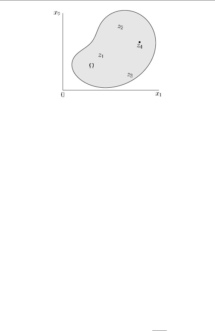
In the inverse problem of interest, the initial condition is unknown. The additional

information is gained in observations performed over the solution at some individual

points in the calculation domain; this information is provided by functions u(x, t )

given at points z

∈ , m = 1, 2,...,M (see Figure 7.17). With regard to the

measurement inaccuracies, we put:

u(z

, t) ≈ ϕ

(t), 0 < t < T, m = 1, 2,...,M. (7.259)

Section 7.5 Continuation of non-stationary ﬁelds from point observation data 327

Figure 7.17 Schematic illustrating the statement of the problem

It is required to ﬁnd, from equation (7.257), boundary conditions (7.258) and addi-

tional measurements (7.259), the function u(x, t).

With the given data measured at individual points (see (7.259)), we can pose a prob-

lem aimed at treating the data. At each time, we can try to interpolate (extrapolate)

these data towards all points in the calculation domain. From this standpoint, the

above-posed inverse problem (7.257)–(7.259) can be considered as a problem in which

it is required to treat the data maximally taking into account a priori information about

the solution; here, the interpolation problem is to be solved in the class of functions

that satisfy equation (7.257) and boundary conditions (7.258).

7.5.2 Variational problem

In the consideration of inverse problem (7.257)–(7.259), we will restrict ourselves to

the cases in which it is required to solve such problems approximately. We will solve

these problems on the basis of the Tikhonov regularization method. To this end, we

will use the formulation of the inverse problem as an optimal control problem.

As the control v(x), it seems reasonable to choose the initial condition. We de-

note the corresponding solution as u(x, t;v). The state u(x, t;v) of the system is

pre-deﬁned by equation (7.257), by boundary conditions (7.258), and by the initial

condition

u(x, 0;v) = v(x), x ∈ . (7.260)

We assume that the control v(x) belongs to the Hilbert space H ={v(x) | v(x) ∈

(), v(x) = 0, x ∈ ∂}, in which the scalar product and the norm are deﬁned as

(v, w) =



v(x)w(x) dx, v=



(v, v).

328 Chapter 7 Evolutionary inverse problems

In line with (7.259), we choose the smoothing functional in the form

(v) =



m=1



(u(z

, t;v) − ϕ

(t))

dt + αv

, (7.261)

where α>0 is the regularization parameter, whose value must be chosen considering

the inaccuracy in the measurements (7.259).

The optimal control w(x) is to be chosen from the minimum of (7.261), i.e.,

(w) = min

v∈H

(v). (7.262)

The solution of the inverse problem is u(x, t) = u(x, t;w).

For the variational problem (7.257), (7.258), (7.260)–(7.262), we use a somewhat

more general differential-operator statement, considering the problem in H, so that

u(x, t;v) = u(t;v) ∈ H. We write equation (7.257) with boundary conditions (7.258)

in H in the form of an evolutionary ﬁrst-order equation:

+ Au = 0, 0 < t < T. (7.263)

The operator A, deﬁned as

Au ≡−



β=1

∂

∂x



k(x)

∂u

∂x



is self-adjoint and positively deﬁned in H:

A = A

∗

≥ κλ

E, (7.264)

where k(x) ≥ κ>0, and λ

> 0 is the minimal eigenvalue of the Laplace operator.

We introduce the function χ ∈ H:

χ =



m=1

δ(x − z

Here, δ(x) is the δ-function, and let ϕ(t) ∈ H be a function such that

χϕ(t) =



m=1

δ(x − z

)ϕ

(t).

With the notation introduced, the functional (7.261) can be rewritten as

(v) =



(χ, (u(t;v) − ϕ(t))

) dt + αv

. (7.265)

Equation (7.263) is supplemented with the initial condition (see (7.260))

u(0) = v. (7.266)

So, we arrive at the minimization problem (7.262), (7.265) for the solutions of problem

(7.263), (7.266).

Section 7.5 Continuation of non-stationary ﬁelds from point observation data 329

7.5.3 Difference problem

For simplicity, we restrict ourselves to the case in which  is a rectangle:

 ={x | x = (x

, x

), 0 < x

< l

,β= 1, 2}.

In the domain , we introduce a grid, uniform over either direction, with grid sizes h

α = 1, 2. Suppose that, as usually, ω is the set of internal nodes.

On the set of mesh functions y(x) such that y(x) = 0, x = ω, by the relation

y =−



β=1

¯x

)

, (7.267)

we deﬁne the difference operator , where, for instance,

(x) = k(x

− 0.5h

, x

), a

(x) = k(x

, x

− 0.5h

In the mesh Hilbert space H = L

(ω), we introduce the scalar product and the norm

with the relations

(y,w) =



x∈ω

y(x)w(x)h

, y=



(y, y).

In H we have  = 

∗

≥ γ E, m > 0, where

γ = κ





From (7.263) and (7.266), we pass to the differential-operator equation

+ y = 0, 0 < t < T (7.268)

with the given initial condition

y(0) = v, x ∈ ω. (7.269)

We denote by y

the difference solution at the time t

= nτ , n = 0, 1,...,N

τ = T , where τ>0 is the time step size. For problem (7.268), (7.269), we will use

the two-layer scheme with the weights

n+1

− y

+ (σ y

n+1

+ (1 − σ)y

) = 0,

n = 0, 1,...,N

− 1,

(7.270)

supplemented with the initial condition

(x) = v(x), x ∈ ω. (7.271)

330 Chapter 7 Evolutionary inverse problems

We write scheme (7.270) in the canonical form

n+1

− y

+ Ay

= 0, n = 0, 1,...,N

− 1. (7.272)

For the difference operators B and A we have:

B = E + στA, A = . (7.273)

The scheme with weights (7.272) and (7.273) in the case of A = A

∗

> 0 is stable

(see Theorem 4.14) in H provided that

E + τ



σ −



A ≥ 0.

This (necessary and sufﬁcient) condition is fulﬁlled for all σ ≥ 0.5, i.e., here we have

an unconditionally stable difference scheme. In the case of σ<0.5 scheme (7.272),

(7.273) is conditionally stable. For the difference solution of problem (7.270), (7.271)

in the case of σ ≥ 0.5 there holds the following a priori estimate:

y

≤v, n = 1, 2,...,N

;

this estimate shows the scheme to be stable with respect to initial data.

We assume that the observation points z

, m = 1, 2,...,M coincide with some

internal nodes of the calculation grid. Like in the continuous case, we deﬁne the mesh

function χ

∈ H as

(x) =



m=1



δ(x − z

) dx,

i.e., χ

∈ H is the sum of the corresponding difference δ-functions. In a similar way,

we can introduce ϕ

(x, t

), x ∈ ω, n = 1, 2,...,N

so that

(x)ϕ

(x, t

) =



m=1



δ(x − z

)ϕ

) dx.

To functional (7.265), we put into correspondence the following difference func-

tional:

(v) =



n=1

(χ

,(y(x, t

;v) − ϕ

(x, t

))

)τ + αv

. (7.274)

The minimization problem

(w) = min

v∈H

(v) (7.275)

is to be solved under constraints (7.270) and (7.271).

Section 7.5 Continuation of non-stationary ﬁelds from point observation data 331

7.5.4 Numerical solution of the difference problem

To approximately solve the discrete variational problem of interest, we will use gra-

dient iteration methods. First, we are goint to derive the Euler equation (optimal-

ity condition) for the variational problem to be approximately solved by the iteration

methods.

To formulate the optimality conditions for problem (7.271), (7.272), (7.274),

(7.275), consider the problem for the increments. From (7.271) and (7.272) we have:

δy

n+1

− δy

+ Aδy

= 0, n = 0, 1,...,N

− 1, (7.276)

δy

= δv. (7.277)

To formulate the problem for the conjugate state ψ

, we multiply equation (7.276)

(scalarwise in H )byτψ

n+1

and calculate the sum over n from 0 to N

−1. This yields

−1



n=0

((Bδy

n+1

,ψ

n+1

) + ((τ A − B)δy

,ψ

n+1

)) = 0. (7.278)

With the constancy and self-adjointness of the operators A and B taken into account,

for the ﬁrst term we have:

−1



n=0

(Bδy

n+1

,ψ

n+1

) =



n=1

(δy

, Bψ

We consider the mesh function ψ

for n = 0, 1,...,N

under the following addi-

tional conditions:

= 0. (7.279)

The second term in (7.278) can be rearranged as

−1



n=0

((τ A − B)δy

,ψ

n+1

) =



n=0

((τ A − B)δy

,ψ

n+1

)



n=1

(δy

,(τA − B)ψ

n+1

) + (δy

,(τA − B)ψ

). (7.280)

Substitution of (7.279) and (7.280) into (7.278) yields the equation



n=0

(δy

,(Bψ

+ (τ A − B)ψ

n+1

)) = (δv, Bψ

). (7.281)

332 Chapter 7 Evolutionary inverse problems

With the form of (7.274) taken into account, we determine the conjugate state from the

difference equation

− ψ

n+1

+ Aψ

n+1

= χ

− ϕ

(x, t

)),

n = N

, N

− 1,...,0,

(7.282)

supplemented with conditions (7.279). Scheme (7.279), (7.282) is stable under the

same conditions as scheme (7.271), (7.272) for the ground state.

From (7.281), for the gradient of (7.274) the following representation can be de-

rived:



(v) = 2



Bψ

+ αv



. (7.283)

With (7.283), the necessary and sufﬁcient condition for the minimum of (7.274) can

be written as

Bψ

+ ταv = 0. (7.284)

For equation (7.284) to be solved, we construct the iteration method.

The iteration algorithm for initial-state correction consists in the following organi-

zation of the computational procedure.

• At a given w

(k is the iteration number), we solve the identiﬁcation problem

for the ground state:

n+1

− y

+ Ay

= 0, n = 0, 1,...,N

− 1,

(x) = w

(x), x ∈ ω.

• Then, we calculate the conjugate state:

− ψ

n+1

+ Aψ

n+1

= 2χ

− ϕ

(x, t

)), n = N

, N

− 1,...,1,

− ψ

+ Aψ

= 0,

= 0, x ∈ ω.

• Next, we reﬁne the initial condition:

k+1

− w

k+1

+ Bψ

+ αw

= 0, x ∈ ω.

Thus, the algorithm is based on the solution of two non-stationary difference problems

and on reﬁnement of the initial condition at each iteration step.

Section 7.5 Continuation of non-stationary ﬁelds from point observation data 333

A second, more attractive possibility is related with the construction of the itera-

tion method of minimized discrepancy functional (with α = 0 in (7.274)). The latter

situation arises when the iteration method is used to solve the equation (see (7.284))

Bψ

= 0. (7.285)

In the case of (7.285), we use the same computational procedure as in the solution of

(7.284). Yet, there are no problems with the special deﬁnition of the regularization

parameter, this circumstance being the major advantage of iteration methods over the

Tikhonov regularization method.

7.5.5 Program

In the program listing presented below, the iteration method for the minimization of

the discrepancy functional is realized (equation (7.285) is solved). In order to make

the problem not too complicated, we have restricted ourselves to the iterative method

of simple iteration, in which

k+1

− w

+ Bψ

= 0, x ∈ ω

and the value of s is set explicitly.

Program PROBLEM14

C PROBLEM14 - CONTINUATION OF NON-STATIONARY FIELDS

C FROM POINT OBSERVATIONS

C TWO-DIMENSIONAL PROBLEM

C ITERATIVE REFINEMENT OF THE INITIAL CONDITION

IMPLICIT REAL

8 ( A-H, O-Z )

PARAMETER ( DELTA = 0.02D0, N1 = 51, N2 = 51,M=101,L=10)

DIMENSION A(13

N2), X1(N1), X2(N2)

+ ,XP(L), YP(L), IM(L), JM(L)

+ ,FF(L), FI(L,M), FID(L,M), FIK(L,M)

COMMON / SB5 / IDEFAULT(4)

COMMON / CONTROL / IREPT, NITER

C PARAMETERS:

C X1L, X2L - COORDINATES OF THE LEFT CORNER;

C X1R, X2R - COORDINATES OF THE RIGHT CIRNER;

C N1, N2 - NUMBER OF NODES IN THE SPATIAL GRID;

C H1, H2 - MESH SIZES OVER SPACE;

C TAU - TIME STEP;

C DELTA - INPUT-DATA INACCURACY LEVEL;

C U0(N1,N2) - INITIAL CONDITION TO BE RECONSTRUCTED;

C XP(L), - COORDINATES OF THE OBSERVATION POINTS;

C YP(L)

C FI(L,M) - SOLUTION AT THE OBSERVATION POINTS;

C FID(L,M) - DISTURBED SOLUTION AT THE OBSERVATION POINTS;

334 Chapter 7 Evolutionary inverse problems

C EPSR - RELATIVE INACCURACY OF THE DIFFERENCE SOLUTION;

C EPSA - ABSOLUTE INACCURACY OF THE DIFFERENCE SOLUTION;

C EQUIVALENCE ( A(1), A0 ),

( A(N+1), A1 ),

( A(2

N+1), A2 ),

( A(9

N+1), F ),

( A(10

N+1), U0 ),

( A(11

N+1), V ),

( A(12

N+1), B ),

X1L = 0.D0

X1R = 1.D0

X2L = 0.D0

X2R = 1.D0

TMAX = 0.025D0

PI = 3.1415926D0

EPSR = 1.D-5

EPSA = 1.D-8

SS = - 2.D0

OPEN (01, FILE = ’RESULT.DAT’)! FILE TO STORE THE CALCULATED DATA

C GRID

H1 = (X1R-X1L) / (N1-1)

H2 = (X2R-X2L) / (N2-1)

TAU = TMAX / (M-1)

DOI=1,N1

X1(I) = X1L + (I-1)

END DO

DOJ=1,N2

X2(J) = X2L + (J-1)

END DO

N=N1

DOI=1,13

A(I) = 0.0

END DO

C DIRECT PROBLEM

C PURELY IMPLICIT DIFFERENCE SCHEME

C INITIAL CONDITION

T = 0.D0

CALL MEGP (XP, YP, IM, JM, L, H1, H2)

CALL INIT (A(10

N+1), X1, X2, N1, N2)

CALL PU (IM, JM, A(10

N+1), N1, N2, FF, L)

DO IP = 1,L

FI(IP,1) = FF(IP)

END DO

DOK=2,M

C DIFFERENCE-SCHEME COEFFICIENTS IN THE DIRECT PROBLEM

CALL FDS (A(1), A(N+1), A(2

N+1), A(9

N+1), A(10

N+1),

+ H1, H2, N1, N2, TAU)

Section 7.5 Continuation of non-stationary ﬁelds from point observation data 335

C SOLUTION OF THE DIFFERENCE PROBLEM

IDEFAULT(1) = 0

IREPT = 0

CALL SBAND5 (N, N1, A(1), A(10

N+1), A(9

N+1), EPSR, EPSA)

C OBSERVATIONAL DATA

CALL PU (IM, JM, A(10

N+1), N1, N2, FF, L)

DO IP = 1,L

FI(IP,K) = FF(IP)

END DO

C DISTURBING OF MEASURED QUANTITIES

DO K = 1,M

DO IP = 1,L

FID(IP,K) = FI(IP,K) + 2.

DELTA

(RAND(0)-0.5)

END DO

C INVERSE PROBLEM

C ITERATION METHOD

IT=0

C STARTING APPROXIMATION

DOI=1,N

A(11

N+I) = 0.D0

END DO

100IT=IT+1

C GROUND STATE

T = 0.D0

C INITIAL CONDITION

DOI=1,N

A(10

N+I) = A(11

N+I)

END DO

CALL PU (IM, JM, A(10

N+1), N1, N2, FF, L)

DO IP = 1,L

FIK(IP,1) = FF(IP)

END DO

DOK=2,M

C DIFFERENCE-SCHEME COEFFICIENTS IN THE DIRECT PROBLEM

CALL FDS (A(1), A(N+1), A(2

N+1), A(9

N+1), A(10

N+1),

+ H1, H2, N1, N2, TAU)

C SOLUTION OF THE DIFFERENCE PROBLEM

IDEFAULT(1) = 0

IREPT = 0

CALL SBAND5 (N, N1, A(1), A(10

N+1), A(9

N+1), EPSR, EPSA)