Stacey F.D., Davis P.M. Physics of the Earth

Подождите немного. Документ загружается.

//FS2/CUP/3-PAGINATION/SDE/2-PROOFS/3B2/9780521873628C17.3D

–

277

– [267–293] 13.3.2008 2:15PM

d

r ð 

 p

: (17:23)

Then, integrating with respect to r from the

deepest point of penetration of a ray, at radius

, to the surface, r

 ¼

pdr

r ð 

 p

: (17:24)

This is Abel’s integral equation, giving ,and

hence V, as a function of r from observed values

of D and p.

The solution of Eq. (17.24) in a convenient

form, known as the Wiechert–Herglotz formula

(e.g. Jeffreys, 1959), is



cosh

1



d ¼ p ln



; (17:25)

where p

is the value of p at D ¼D

, for the ray that

penetrates to radius r

, at which the wave speed is

. Equation (17.25) can be used for numerical

integration over any range for which p(D)isa

continuous, monotonic function, and so gives

V(r) over this range. Different seismic phases

give overlapping ranges, allowing interpolation

over the breaks. For example, the major break in

P-wave travel times is due to the core shadow

zone, and since no direct P-waves ‘bottom out’

in the outer part of the core, they cannot indicate

the velocities there. However, SKS-waves involve

much shallower refractions into the core and are

of interest in examining a suggestion that there is

a gravitationally stable layer at the top of the core

(Section 22.7).

The PREM earth model (Appendix F) relies

heavily on free oscillation periods, but the models

that pre-dated free oscillation observations were

based entirely on body wave travel times and were

quite close to the currently accepted structure.

The modern model, ak135, uses this approach.

17.5 Earth models: density variation

in a homogeneous layer

Observations of the speeds of both P- and S-

waves, V

and V

, Eqs. (16.1) and (16.2), allow

/ and K/ to be determined:

 ¼ K= ¼ V



; (17:26)

= ¼ V

; (17:27)

but without further information density, , can-

not be estimated independently. Earth models

based entirely on body wave data were con-

structed by assuming large regions, where body

wave speeds are smoothly varying, to be chemi-

cally and mineralogically homogeneous. Then

the density increases with depth, z, by hydro-

static compression,



d



g ¼

g



; (17:28)

where P is the pressure and g is gravity.  is a

known function of depth by Eq. (17.26), but g

depends on the density profile itself, since

g ¼ GmðrÞ=r

; (17:29)

where G ¼6.674 10

11

1

2

is the gravi-

tational constant and m(r) is the total mass inside

radius r,

mðr Þ¼

4pr

ðrÞdr: (17:30)

Equation (17.28) is the Williamson–Adams

equation for the density profile in a homo-

geneous layer. It is commonly referred to as

the Adams–Williamson equation, although

E. D. Williamson is the first author of the now

rather obscure paper in which it first appeared.

Since the compressions and rarefactions of

seismic waves are adiabatic, the incompressi-

bility in Eq. (17.26) is the adiabatic value, K

Therefore, when this is used in Eq. (17.28), the

density variation represented by this equation is

that due to adiabatic compression. It gives the

density gradient in a homogeneous layer with an

adiabatic temperature gradient. The most exten-

sive, apparently homogeneous regions within

the Earth, the outer core and the lower mantle,

are believed to support temperature gradients

that are close to adiabatic, so Eq. (17.28) applies

directly to these regions, with a minor proviso

concerning granular materials, considered

below. If the temperature gradient differs from

the adiabatic value by an amount

17.5 DENSITY VARIATION 277

//FS2/CUP/3-PAGINATION/SDE/2-PROOFS/3B2/9780521873628C17.3D

–

278

– [267–293] 13.3.2008 2:15PM

 ¼





Adiabatic

; (17:31)

then a correction term is applied to Eq. (17.28),

d

g



 ; (17:32)

where  is the volume expansion coefficient. This

is Birch’s generalization of the Williamson–Adams

equation (Problem 17.6). In the lithosphere, where

the average excess temperature gradient is of

order 10

2

1

(10 8C/km) the two terms in

Eq. (17.32) are of comparable magnitudes

(Problem 19.3). The correction term is believed to

be significant also in the layer D

,atthebaseofthe

mantle.

Equation (17.28), without the added term in

Eq. (17.32), must apply very precisely to the outer

core, which is homogeneous and adiabatic. Apart

from the lithosphere and the D

layer, and thermal

complications in the phase transition zone

(Section 22.5), most of themantleisbelievedto

be quite close to adiabatic. As we point out

below, this is the conclusion to the application of

Eq. (17.32) to the lower mantle, but in Section 12.6

we point out that different regions of the mantle,

especially the lower mantle, must be convectively

cooled sequentially, and not simultaneously, so

that some heterogeneity is inevitable.

There are two other effects that complicate

the picture in the lower mantle. One is observa-

tionally indistinguishable from a departure from

adiabatic conditions, and applies to granular

materials, such as rocks with minerals having

different elasticities. It is a consequence of the

difference between relaxed and unrelaxed mod-

uli, as discussed in Section 10.4. The unrelaxed

modulus, K

VRH

in Eq. (10.13), deduced from seis-

mic wave speeds, is slightly higher than the

relaxed modulus K

in Eq. (10.12), which governs

static compression. For the lower mantle min-

eral mix the difference is listed in Table 18.1.

When Eq. (17.32) is used to infer the departure

from an adiabatic gradient, , a correction to  is

required to convert the unrelaxed modulus

observed seismologically to the smaller relaxed

modulus. Failure to apply this correction leads to

a value of  that is too small. Over the depth

range of the lower mantle this leads to a 100 K

underestimate of the temperature difference. A

temperature increment of 100 K, in excess of the

adiabat across the lower mantle, is inferred if

Eq. (17.32) is used with uncorrected PREM data.

The correction to the relaxed modulus increases

this increment to 200 K (Stacey, 2005).

Another complication that prevents precise

fitting of the Williamson–Adams equation to

the lower mantle arises from a subtle electronic

phase transition in iron ions at lower mantle

pressures. As discussed in Section 18.9, this

transition is smeared over a wide pressure

range, possibly almost the entire lower mantle.

As for all pressure-induced transitions, the high-

pressure state has higher bulk modulus and

density, so that there is a slightly greater, but

gradual, increase in density with depth than

would be expected for constant phase material

and there is an ‘anomalous’ contribution to

dK/dP. The departure of the lower mantle

from the Williamson–Adams equation is never-

theless quite modest, but inferences such as

departure from the adiabat must be treated

with caution.

17.6 Internal structure of the

Earth: the broad picture

The first step in elucidating the structure of the

Earth was the identification of the major layers

and the depths of the boundaries between them.

The radial variation in velocity, obtained from

body waves and shown in Fig. 17.9, accom-

plished this. Additional information is needed

to deduce the density variation. Frequencies of

numerous modes of free oscillation are well

observed and the spheroidal modes involve grav-

itational restoring forces, so inversion of the free

mode spectrum allows the development of a

complete model, including the density profile.

However, inversion calculations need a starting

point and this was provided by models based on

body wave data and constrained to match the

mass and moment of inertia of the Earth.

The crust is the only part of the Earth for

which density can be measured directly.

However, the isostatic balance of large surface

278 SEISMOLOGICAL DETERMINATION OF EARTH STRUCTURE

//FS2/CUP/3-PAGINATION/SDE/2-PROOFS/3B2/9780521873628C17.3D

–

279

– [267–293] 13.3.2008 2:15PM

features, such as mountain ranges and conti-

nents, allows the density of the uppermost part

of the mantle to be calculated, as considered in

Section 9.3, (see Fig. 9.6). The value is close to

3370 kg m

3

. Studies of upper mantle-derived

rocks confirm that this is a reasonable estimate.

It provides a starting point for downward extra-

polation of density by Eq. (17.28) or (17.32). This

extrapolation can be extended as far as the veloc-

ity structure indicates that homogeneity is a rea-

sonable assumption, but in the upper mantle a

series of velocity increments intervenes.

If we make the simplifying assumption that

below the upper mantle there are only two

regions, the lower mantle and the core, and

that each of these is homogeneous and adiabatic,

then Eq. (17.28) applies through each of them. In

this case we need to specify only the density at

any one level in each and these densities must be

selected so that the total mass and moment of

inertia of the model match the values of the

Earth (Eq. (7.3)). The use of moment of inertia

was a vital step in model calculations in the

1930s and 1940s by K. E. Bullen, who showed

that the lower mantle was intrinsically more

dense than the uppermost mantle by about

700 kg m

3

. He therefore identified the upper

mantle velocity increments (Fig. 17.9), that we

now explain as due primarily to recognized

phase transitions in silicates, with a zone of

increasing density. The models developed on

this basis were remarkably close to our present

ideas on Earth structure, as summarized in

Appendix F.

Earth models derived from both free oscilla-

tion and body wave data are necessarily more

secure than models based on one of these data

sets alone. The two types of observation each

have advantages and limitations. The free

modes give accurate global average properties,

but have long wavelengths that cannot distin-

guish fine details, such as whether boundaries

are sharp. Body waves can be used to examine

details that are inaccessible to free oscillation

studies, including lateral heterogeneities, but

do not lead directly to density estimates. In con-

sidering free oscillations and body waves

together, a wide range of frequencies is involved,

from 0.3 mHz for the

mode to more than

1 Hz for high frequency body waves. Over

this frequency range dispersion is significant

(Section 10.7) and must be allowed for, which

means that, although Q has the character of a

minor correction factor, it is an essential param-

eter in detailed Earth models.

Appendix F gives selected details of the most

widely used earth model, which is known by its

acronym, PREM (Preliminary Reference Earth

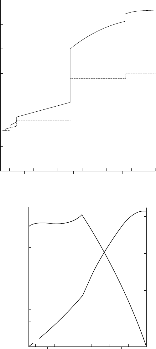
Model). The density structure is plotted in

Fig. 17.11(a), with corresponding values of inter-

nal pressure and gravity in Fig. 17.11(b). The

seismic velocities do not differ, to an extent

that is noticeable on a graph, from those of the

ak135 model, referred to in Section 17.4. PREM

includes dispersion corresponding to a simple Q

structure, inferred from free oscillations, and

assumed to be uniform over broad depth ranges

and to be frequency-independent. This means

dispersion given by Eq. (10.29), which, as sug-

gested in Section 10.7, probably overestimates

the dispersion in the Earth because Q shows a

general increase with frequency. The details in

Appendix F refer to properties at 1 Hz. PREM is a

global average model, a reference structure for

studies of finer details, including lateral hetero-

geneities, and for discussions of the physics of

the deep interior. Anisotropy of the upper layers

and separate continental and oceanic structures

are given in the original tabulation (Dziewonski

and Anderson, 1981).

17.7 Boundaries and discontinuities

Lateral velocity variations are recognized, but

are generally small compared with the radial

variations displayed in Fig. 17.9. There is a gen-

eral increase with depth due to the pressure

dependence of elasticity, but with discontinu-

ities in radial structure that must be explained

in terms of layers with different compositions

and/or crystal structures. Important questions

about a boundary between layers that can be

answered by seismological studies are

(i) what are the differences in the properties

(densities, elasticities) of the materials

above and below the boundary?

17.7 BOUNDARIES AND DISCONTINUITIES 279

//FS2/CUP/3-PAGINATION/SDE/2-PROOFS/3B2/9780521873628C17.3D

–

280

– [267–293] 13.3.2008 2:15PM

Depth (km)

Gravity, g

–2

)

1000 2000 3000 4000 5000 6000 6371

6000 5000 4000 3000 2000 1000

0.5

1.5

2.5

3.5

Radius (km)

Pressure, P

(10

Pa)

FI G U R E 17.11(b) Gravity and pressure

corresponding to the density profile in

Fig. 17.11(a).

6000 5000 4000 3000 2000 1000 0

0 1000 2000 3000 4000 5000 6371

6000

Depth (km)

Radius (km)

Density (1000 kg m

–3

)

FI G U R E 17.11(a) Profile of

density, , for the earth model

PREM with corresponding zero

pressure, low temperature

density, estimated by finite strain

theory (Chapter 18).

280 SEISMOLOGICAL DETERMINATION OF EARTH STRUCTURE

//FS2/CUP/3-PAGINATION/SDE/2-PROOFS/3B2/9780521873628C17.3D

–

281

– [267–293] 13.3.2008 2:15PM

(ii) is the boundary universal or does it occur

only in particular areas?

(iii) is it sharp or diffuse?

(iv) is it smooth, undulating or rough?

The contrast in properties across each of the

important boundaries in the Earth, as determined

in model studies, is unambiguous where the

boundaries are sharp and isolated from one

another and from graded transitions. A check

that these conditions are satisfied is provided by

measurements of reflection coefficients and P to

SV or SV to P conversions. Reflections occur only

where a boundary is sharp, relative to the wave-

length used to investigate it. Thus, a boundary

that has a reflection coefficient, independent of

frequency up to the highest usable frequency, is

sharp in the sense of having no observable struc-

ture. The core–mantle boundary (CMB) is the

most obvious example. This is a boundary

between liquid metal and solid, rocky material.

However, many reflections from it are very weak

because the reflection coefficient is determined

by the contrast in acoustic impedance, velocity 

density, which for P-waves happens to be nearly

the same in the core and mantle (see Problem

16.1, Appendix J). The inner core boundary

(ICB) is also found to be sharp (less than 2 km

thick according to Kawakatsu, 2006), allowing

no more than a thin mushy zone where outer

core fluid is freezing out. Reflections observed in

the mantle, especially at the 410 and 670 km

boundaries, are attributed to solid–solid phase

transitions between different mineral assemb-

lages (Tables 2.4a,b). Not all such transitions

are sharp. Graded transitions can be observed

only by seismic refractions, that is by travel-time

studies.

Some boundaries occur at different depths in

different areas or are seen in some areas but are

missing from others. The boundary between the

crust and mantle, the Mohorovic

discontinuity,

M layer or Moho, is typically 7 km below the sea

floor in oceanic areas, but 35 to 40 km deep

under continents and 60 km under major moun-

tain ranges. The different crustal thicknesses are

isostatically balanced (Section 9.3) and so the

seismological observation of the Moho depth

gives a measure of the density contrast between

the crust and mantle. Similar undulations of the

core–mantle boundary have been sought, but are

relatively slight (Doornbos and Hilton, 1989), the

strong heterogeneities at the boundary being

attributable to the base of the mantle (layer D

In the case of the CMB the height and typical

wavelength of the undulations are important to

the mechanical coupling of the mantle to core

motions (Section 7.5).

In Section 12.5 the irregularities in D

are

attributed to a structure analogous to continents

and ocean basins at the surface (Fig. 12.3). Young

and Lay (1990) reported evidence of a boundary

at about 250 km above the CMB and it appears

possible that this is an upper boundary of a

crypto-continent (see Fig. 12.3). This boundary

is observed in some areas, but appears to be

absent from others, which are therefore

assumed to be crypto-oceanic areas where ‘nor-

mal’ mantle extends down to the CMB. It will

be important to our understanding of the

core–mantle interaction to determine what frac-

tion of the CMB is of each kind. The distinction

is, in any case, compromised by the transition to

the post-perovskite phase near to the base of the

mantle. Undulations of this phase boundary

would arise from the temperature dependence

of the transition pressure.

Recent analysis of digital seismic data have

revealed patches of extremely low velocity at the

base of the D

region at the CMB. The origin of

these so-called ultra low velocity zones (ULVZs) is

controversial, with explanations ranging from

temperature effects, possibly accompanied by

partial melt, to variations in composition as sili-

cate material interacts with the iron of the core.

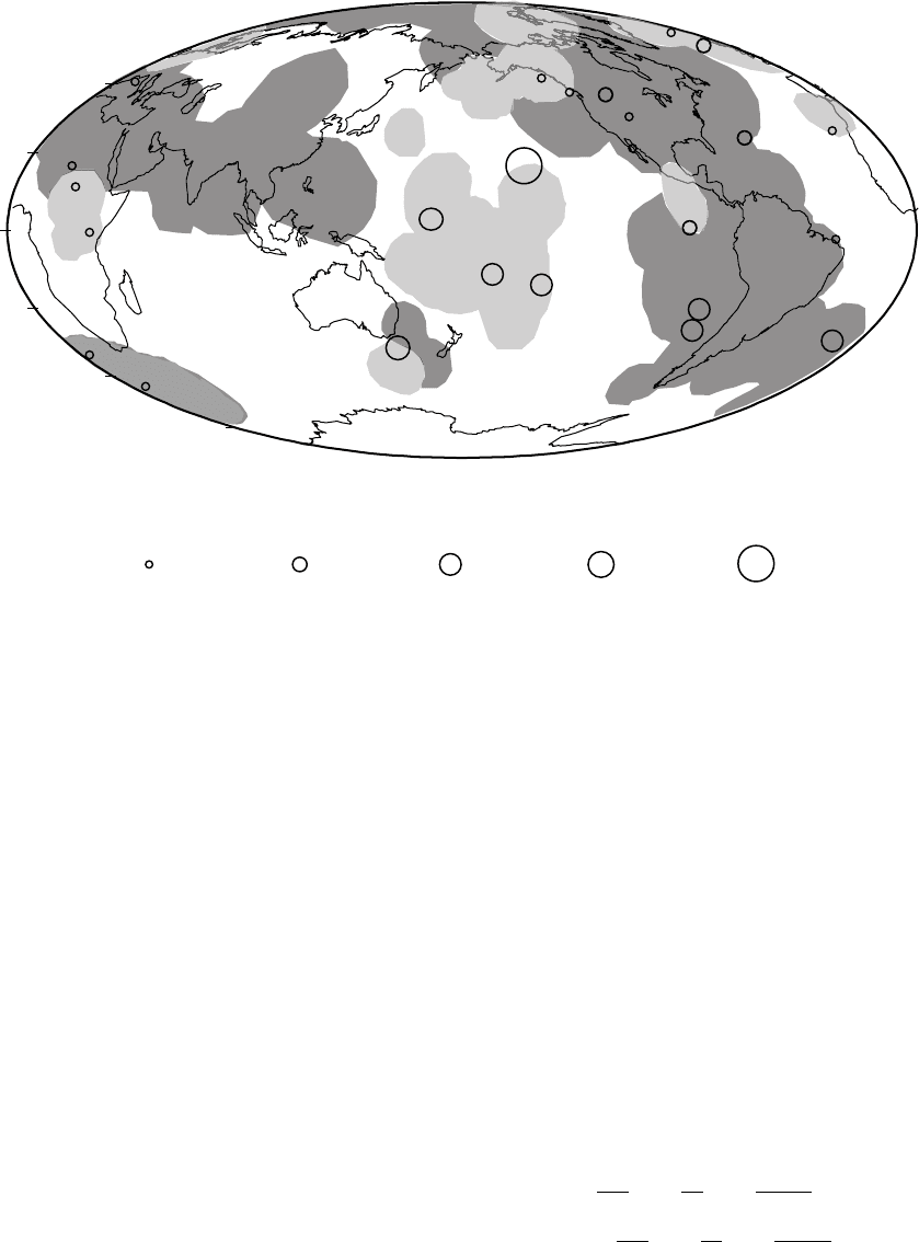
Maps of ULVZs (Fig. 17.12) correspond roughly

to the distribution of hot spots and so ULVZs may

be the bases of plumes upwelling from the core–

mantle boundary to the surface (Williams et al.,

1998). The alternative explanation is that the

post-perovskite mineral phase (ppv) at the base

of the mantle absorbs iron from the core and

iron-rich ppv has low seismic velocities, consistent

with ULVZs (Mao et al., 2006).

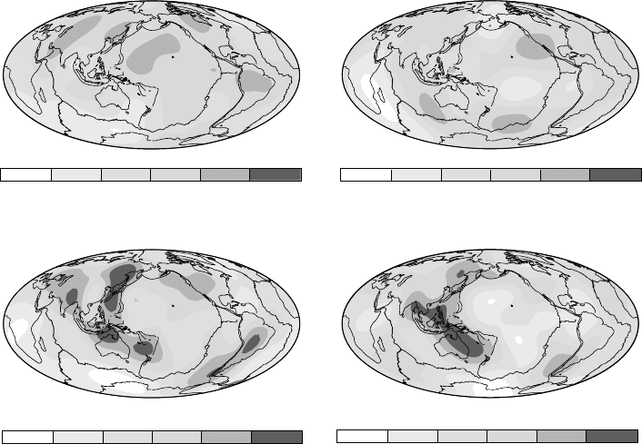
Topographic maps of the 410 and 660 km dis-

continuities (Fig. 17.13) show that they undulate

by 20 km or more in depth (Flanagan and Shearer,

1998). For the pyrolite model of mantle minerals

17.7 BOUNDARIES AND DISCONTINUITIES 281

//FS2/CUP/3-PAGINATION/SDE/2-PROOFS/3B2/9780521873628C17.3D

–

282

– [267–293] 13.3.2008 2:15PM

the 410 km boundary marks the  !  transi-

tion of olivine and the 660 km boundary marks

the transition to perovskite þmagnesiowustite.

Clapeyron slopes, dT

/dP, for the phase transi-

tions are positive for the 410 km transition and

negative for that at 660 km, so that the boundary

undulations would be negatively correlated if

caused by temperature only. This is not always

clear (Flanagan and Shearer, 1998) but evidence

of regions exhibiting negative correlation is

accumulating. At subduction zones the 660 km

boundary is found to be deeper than the global

average, but correlated shallowing of the 410 km

boundary is not easily observed, perhaps because

it is more localized to the slab and presents too

limited an area for seismic reflections. Lebedev

et al. (2002) used seismically estimated variations

in transition zone depths and thicknesses, H,

beneath stations in Australia and East Asia and

temperatures estimated from tomography to

obtain Clapeyron slopes. Differential arrival

times of P–S converted phases from the 660 km

and 410 km discontinuities were converted to H

using the tomographic velocities. Temperatures

at the discontinuities were inferred by using labo-

ratory estimates of ð@ ln V

=@T Þ

to convert veloc-

ity variation,  ln V

, to temperature. A plot of T

versus H has a slope dT/dH ¼0.13 0.07 km/K, in

agreement with the laboratory value for pyrolite,

0.13 km/K (Bina and Helffrich, 1994). Variation in

transition zone thickness is

H ¼



660



660

@ ln V



 ln V

660





410



410

@ ln V



 lnV

410

(17:33)

<0.5

0.6

– 1.5

1.6

– 2.5

2.6

– 3.5 >3.6

Hot spot flux (Mg/s)

FI G U R E 17.12 Locations of ultra low velocity zones (ULVZs) at the base of the mantle. Light shading shows

where they are more than 5 km thick, dark shading indicates their absence, or thicknesses less than 5 km. Areas

where no determinations have been made are unshaded. Circles represent hot spots with symbol size being

proportional to estimated strength in areas studied, and crosses indicating hot spots above regions

not yet seismically investigated for ULVZs. (Redrawn from Williams et al., 1998.)

282 SEISMOLOGICAL DETERMINATION OF EARTH STRUCTURE

//FS2/CUP/3-PAGINATION/SDE/2-PROOFS/3B2/9780521873628C17.3D

–

283

– [267–293] 13.3.2008 2:15PM

Data from multiple stations and events were

used to estimate ðdP=dT

410

¼ð2  2 MPa=KÞ

and ðdP=dT

660

¼ð3  1:5 MPa=KÞ separately.

These values, although imprecise, are compati-

ble with the range of laboratory estimates.

Evidence of an upper mantle boundary

520 km from the surface was seen in stacked dig-

ital records of reflected waves by Shearer (1990).

This boundary does not appear in PREM. It must

occur at a more or less fixed depth to be seen in

the globally stacked records, but in regional

stacked records this transition has proved to be

more elusive. Deuss and Woodhouse (2001) found

that in some places the 520 km boundary appears

as a single reflector, whereas in others it is either

split or not visible at all. Possible candidates are

the   transition in the olivine component and

the garnet–perovskite transition in the non-

olivine component (Ita and Stixrude, 1992).

With variations in temperature or composition

these could occur at significantly different

depths. A systematic relationship between split-

ting and tomographic velocity, which would be

expected if temperature effects dominate, has

not been observed, indicating that composition

is also important. The 520 km phase transition is

evidently spread over a greater depth range

(10 km) than the 410 or 660 km transitions

(2 km) because it does not reflect short period

energy (Benz and Vidale, 1993). Its absence from

PREM and from refraction studies (Jones et al.,

1992) suggests that it arises from a density incre-

ment (but not a sharp one), with little velocity

change, giving an impedance mismatch and

consequent reflections of long-period waves at

near-vertical incidence, but little indication in

refractions or short-period observations (Rigden

et al., 1991; Vidale, 2001).

The boundary at about 200 km (180 km in

PREM) was not seen in Shearer’s (1990) analyses.

These discrepancies suggest fundamental dif-

ferences between the boundaries, their depend-

ences on temperature and composition and

between methods of observation. The boundary

at 180 km in PREM is the base of a low-velocity

zone, which we identify with the asthenosphere

or soft layer of the upper mantle. It is less well

developed under continents than under oceans,

and if it occurs at a variable depth, when seis-

mograms from different wave paths are added

‘410’ ‘520’

400 406 412 418 424 430 436 497 503 509 515 521 527 533

‘660’ TZ Thickness

Depth (km)

642 648 654 660 666 672 678 223 229 235 241 247 253 259

FI G U R E 17.13 Undulations of phase boundaries and transition zone thickness (Flanagan and Shearer, 1998).

17.7 BOUNDARIES AND DISCONTINUITIES 283

//FS2/CUP/3-PAGINATION/SDE/2-PROOFS/3B2/9780521873628C17.3D

–

284

– [267–293] 13.3.2008 2:15PM

inthestackingprocess,evidenceforadisconti-

nuity is washed out.

17.8 Lateral heterogeneity: seismic

tomography

Lateral heterogeneities are most obvious in the

crust andoccur throughoutthemantle. As pointed

out in Section 17.1, the outer core must be very

homogeneous. It is difficult to imagine significant

compositional heterogeneity in the inner core,

but its anisotropy is probably quite variable; in

any case, seismology gives rather poor resolution.

Lateral structure is explored in various ways, espe-

cially by seismic tomography. Tomography is a

word borrowed from the medical imaging of ana-

tomical structure by multi-directional X-rays, but

the analogy is imperfect because X-ray imaging

depends entirely on variations in absorption,

with no refraction or diffraction. Seismic tomog-

raphy relies on variations in wave velocity, so that

body waves arriving early (or late), relative to

waves through a reference model such as PREM,

have traversed faster (or slower) paths than aver-

age. Travel times over numerous paths in various

directions allow the heterogeneities to be local-

ized. But the resolution is limited by the neglect

of diffraction (Doornbos, 1992).

The propagation of seismic waves is, in many

respects, analogous to the propagation of light

waves. Although the similarity includes diffraction,

there is an important difference between the way

we view diffracted light and the treatment of most

seismic signals. When we see an optical diffraction

pattern we are looking at the effect of a continuous

(usually monochromatic) wave. Light arriving at

any point in the field of view is, in general, a phased

sum of the contributions from several paths of

various optical lengths. In travel-time tomography

we consider only the first arrivingpulse, which

means that we use only the component of the

signal that travels by the fastest path. As

mentioned in Sections 16.1 and 16.3, Wielandt

(1987) drew attention to problems that can arise

in the identification of low- or high-velocity regions

from the arrival times of seismic pulses propagat-

ing through or diffracted around them.

Consider first a low-velocity sphere. Beyond a

limited distance, determined by the size and

velocity contrast, the wave diffracted around it

arrives earlier than the wave directly through it

and the anomaly becomes seismically invisible.

For a sphere of high-velocity material, the direct

transmitted wave arrives first and the sphere

remains visible to much greater distances.

Refraction by the sphere spreads out the trans-

mitted early wavefront, so that eventually it is

lost, but at intermediate distances the wave

spreading has the effect of making the anoma-

lous volume appear larger than it is. Thus, body

wave travel times lead to overestimates of high-

velocity anomalies and underestimates of low-

velocity anomalies. Tomography can only

identify broad features in the deep mantle.

Some of the things that would be of interest,

especially small low-velocity features, such as

the stems of ascending plumes, are inaccessible.

High-velocity features, such as fragments of sub-

ducted slabs, are more visible. On the present

evidence it is difficult to judge the importance

of the tendency for globally averaged body wave

speeds to be biased high.

Recognizing these limitations, travel-time

tomography, using high-frequency body waves,

has been applied to large-scale features in the

lower mantle (Dziewonski, 1984), yielding

anomalies with velocity contrasts up to 1%. The

spatial pattern was represented by harmonic

degrees up to 6, sufficient to outline features

about 2000 km across. Subsequent analyses con-

firmed that at least the larger-scale features are

robust, although they are regional averages of

structures with unseen finer details. Studies of

upper mantle tomography (Woodhouse and

Dziewonski, 1984; Zhang and Tanimoto, 1991,

1992) used surface waves with numerous inter-

locking paths. The principle is similar except

that, for any wave path, the different depths

are sampled by comparing different frequency

ranges (Section 16.5). Subsequent to these early

studies, numerous global tomographic models

have been presented (e.g., Grand et al., 1997;

Grand, 2001; Su and Dziewonski, 1997; Ritsema

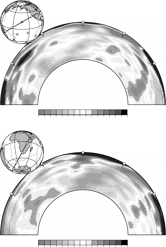
et al., 1999 – see Fig. 17.14(a); Masters et al., 2000 –

see Figs. 17.14(b)–(d)) for which there has been a

general convergence on locations and sizes of

284 SEISMOLOGICAL DETERMINATION OF EARTH STRUCTURE

//FS2/CUP/3-PAGINATION/SDE/2-PROOFS/3B2/9780521873628C17.3D

–

285

– [267–293] 13.3.2008 2:15PM

mantle heterogeneities. Of particular note is the

discovery that some parts of the subducting slabs

beneath North and South America can be traced

through the mantle transition zones all the way to

the core (Fig 17.14(a)), effectively ending a debate

about isolation of the convective circulations of

the upper and lower mantles. Some slabs in the

western Pacific and beneath Asia appear to pond

–1.5% +1.5%

shear velocity variation from 1-D

Latitude

= 20°

Longitude

= –155° Azimuth = 60°

(–)

(+)

–1.5% +1.5%

shear velocity variation from 1-D

(–)

(+)

Latitude

= –30°

Lon

itude = 20° Azimuth = 28°

FI G U R E 17.14(a) Cross-sections of a seismic tomography model (Ritsema et al., 1999), showing Pacific and African

superplumes and deep subduction of the Farallon plate under the Americas.

17.8 LATERAL HETEROGENEITY: SEISMIC TOMOGRAPHY 285

//FS2/CUP/3-PAGINATION/SDE/2-PROOFS/3B2/9780521873628C17.3D

–

286

– [267–293] 13.3.2008 2:15PM

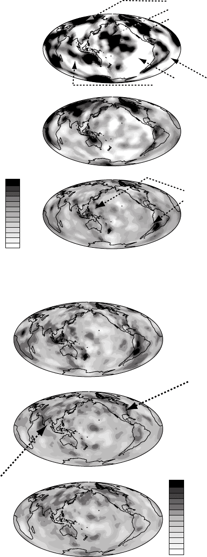
SB4L18-Upper Mantle

60 km

290

700

2.2

1.4

0.6

–0.6

–1.4

–2.2

slow mid-ocean ridges

fast continental shield

and old oceans

the continental plates have fast

'keels' at depths at which the

oceanic areas are already underlain

by the slow asthenosphere

The 'cold' subducting slabs show up

as seismically fast areas. They pass the

660

km discontinuity between upper and

lower mantle and penetrate well into

the lower mantle.

δ Vs/Vs

[%]

SB4L18-Mid-Mantle

Some of the 'cold' subducting slabs

can be traced well into the lower mantle.

E.g. old Farallon and Tethian subducting

slabs.

2.2

1.4

0.6

–0.6

–1.4

–2.2

δ Vs/Vs

[%]

925

1525

1825

FIGURE 17.14 (b), (c) Map views of mantle tomograms from Masters et al. (2000).

Figures provided by Gabe Laske

286 SEISMOLOGICAL DETERMINATION OF EARTH STRUCTURE