Stewart J. Calculus

Подождите немного. Документ загружается.

In the second case , we get

and, putting this in Equation 5, we have . So we have to

solve the cubic equation

Using a graphing calculator or computer to graph the function

as in Figure 6, we see that Equation 7 has three real roots. By zooming in, we can ﬁnd

the roots to four decimal places:

(Alternatively, we could have used Newton’s method or a rootﬁnder to locate these

roots.) From Equation 6, the corresponding -values are given by

If , then x has no corresponding real values. If , then

. If , then . So we have a total of ﬁve critical

points, which are analyzed in the following chart. All quantities are rounded to two

decimal places.

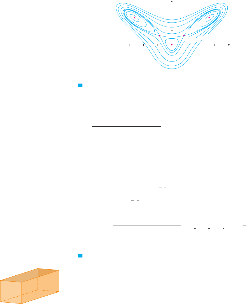
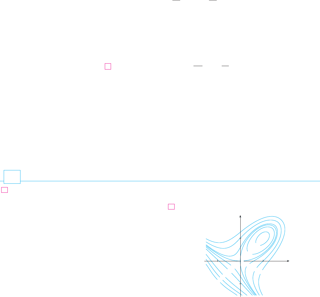
Figures 7 and 8 give two views of the graph of and we see that the surface opens

downward. [This can also be seen from the expression for : The dominant terms

are when and are large.] Comparing the values of at its local maxi-

mum points, we see that the absolute maximum value of is . In

other words, the highest points on the graph of are .

FIGURE 7 FIGURE 8

共⫾2.64, 1.90, 8.50兲f

f 共⫾2.64, 1.90兲⬇8.50f

ⱍ

ⱍⱍ

ⱍ

⫺x

⫺ 2y

f 共x, y兲

x ⬇ ⫾2.6442y ⬇ 1.8984x ⬇ ⫾0.8567

y ⬇ 0.6468y ⬇ ⫺2.5452

x 苷 ⫾

5y ⫺ 2.5

y ⬇ 1.8984 y ⬇ 0.6468 y ⬇ ⫺2.5452

t共y兲苷 4y

⫺ 21y ⫹ 12.5

⫺ 21y ⫹ 12.5 苷 0

25y ⫺ 12.5 ⫺ 4y ⫺ 4y

苷 0

苷 5y ⫺ 2.5

共10y ⫺ 5 ⫺ 2x

苷 0兲

962

||||

CHAPTER 15 PARTIAL DERIVATIVES

Critical point Value of D Conclusion

0.00 ⫺10.00 80.00 local maximum

8.50 ⫺55.93 2488.72 local maximum

⫺1.48 ⫺5.87 ⫺187.64 saddle point共⫾0.86, 0.65兲

共⫾2.64, 1.90兲

共0, 0兲

FIGURE 6

_3 2.7

Visual 15.7 shows several families

of surfaces.The surface in Figures 7 and 8

is a member of one of these families.

TEC

EXAMPLE 5 Find the shortest distance from the point to the plane

SOLUTION The distance from any point to the point is

but if lies on the plane , then and so we have

. We can minimize by minimizing the simpler

expression

By solving the equations

we ﬁnd that the only critical point is . Since , , and , we

have and , so by the Second Derivatives Test

has a local minimum at . Intuitively, we can see that this local minimum is actually

an absolute minimum because there must be a point on the given plane that is closest to

. If and , then

The shortest distance from to the plane is . M

EXAMPLE 6 A rectangular box without a lid is to be made from 12 m of cardboard.

Find the maximum volume of such a box.

SOLUTION Let the length, width, and height of the box (in meters) be , , and , as shown

in Figure 10. Then the volume of the box is

We can express as a function of just two variables and by using the fact that the

area of the four sides and the bottom of the box is

2xz ⫹ 2yz ⫹ xy 苷 12

yxV

V 苷 xyz

zyx

x ⫹ 2y ⫹ z 苷 4共1, 0, ⫺2兲

d 苷

共x ⫺ 1兲

⫹ y

⫹ 共6 ⫺ x ⫺ 2y兲

苷

(

)

⫹

(

)

⫹

(

)

苷

y 苷

x 苷

共1, 0, ⫺2兲

(

)

⬎ 0D共x, y兲苷 f

⫺ 共 f

兲

苷 24 ⬎ 0

苷 10f

苷 4f

苷 4

(

)

苷 2y ⫺ 4共6 ⫺ x ⫺ 2y兲苷 4x ⫹ 10y ⫺ 24 苷 0

苷 2共x ⫺ 1兲 ⫺ 2共6 ⫺ x ⫺ 2y兲苷 4x ⫹ 4y ⫺ 14 苷 0

苷 f 共x, y兲苷共x ⫺ 1兲

⫹ y

⫹ 共6 ⫺ x ⫺ 2y兲

dd 苷

共x ⫺ 1兲

⫹ y

⫹ 共6 ⫺ x ⫺ 2y兲

z 苷 4 ⫺ x ⫺ 2yx ⫹ 2y ⫹ z 苷 4共x, y, z兲

d 苷

共x ⫺ 1兲

⫹ y

⫹ 共z ⫹ 2兲

共1, 0, ⫺2兲共x, y, z兲

x ⫹ 2y ⫹ z 苷 4

共1, 0, ⫺2兲

FIGURE 9

_10

_20

_30

_1.48

_0.8

SECTION 15.7 MAXIMUM AND MINIMUM VALUES

||||

963

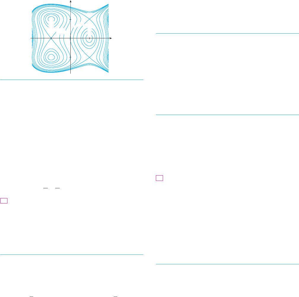
N The ﬁve critical points of the function in

Example 4 are shown in red in the contour map

of in Figure 9.f

N Example 5 could also be solved using

vectors. Compare with the methods of

Section 13.5.

FIGURE 10

Solving this equation for , we get , so the expression for

becomes

We compute the partial derivatives:

If is a maximum, then , but or gives , so we

must solve the equations

These imply that and so . (Note that and must both be positive in this

problem.) If we put in either equation we get , which gives ,

, and .

We could use the Second Derivatives Test to show that this gives a local maximum

of , or we could simply argue from the physical nature of this problem that there must

be an absolute maximum volume, which has to occur at a critical point of , so it must

occur when , , . Then , so the maximum volume of

the box is 4 m . M

ABSOLUTE MAXIMUM AND MINIMUM VALUES

For a function of one variable the Extreme Value Theorem says that if is continuous

on a closed interval , then has an absolute minimum value and an absolute maxi-

mum value. According to the Closed Interval Method in Section 4.1, we found these by

evaluating not only at the critical numbers but also at the endpoints and .

There is a similar situation for functions of two variables. Just as a closed interval con-

tains its endpoints, a closed set in is one that contains all its boundary points. [A bound-

ary point of D is a point such that every disk with center contains points in D

and also points not in D.] For instance, the disk

which consists of all points on and inside the circle , is a closed set because it

contains all of its boundary points (which are the points on the circle ). But if

even one point on the boundary curve were omitted, the set would not be closed. (See

Figure 11.)

A bounded set in is one that is contained within some disk. In other words, it is

ﬁnite in extent. Then, in terms of closed and bounded sets, we can state the following coun-

terpart of the Extreme Value Theorem in two dimensions.

EXTREME VALUE THEOREM FOR FUNCTIONS OF TWO VARIABLES If is continu-

ous on a closed, bounded set in , then attains an absolute maximum value

and an absolute minimum value at some points and

in .D共x

, y

兲

共x

, y

兲f 共x

, y

兲f 共x

, y

兲

f⺢

⺢

⫹ y

苷 1

⫹ y

苷 1

D 苷兵共x, y兲

ⱍ

⫹ y

艋 1其

共a, b兲共a, b兲

⺢

baf

f关a, b兴

V 苷 2 ⴢ 2 ⴢ 1 苷 4z 苷 1y 苷 2x 苷 2

z 苷共12 ⫺ 2 ⴢ 2兲兾关2共2 ⫹ 2兲兴苷 1y 苷 2

x 苷 212 ⫺ 3x

苷 0x 苷 y

yxx 苷 yx

苷 y

12 ⫺ 2xy ⫺ y

苷 012 ⫺ 2xy ⫺ x

苷 0

V 苷 0y 苷 0x 苷 0⭸V兾⭸x 苷 ⭸V兾⭸y 苷 0V

⭸V

⭸y

苷

共12 ⫺ 2xy ⫺ y

兲

2共x ⫹ y兲

⭸V

⭸x

苷

共12 ⫺ 2xy ⫺ x

兲

2共x ⫹ y兲

V 苷 xy

12 ⫺ xy

2共x ⫹ y兲

苷

12xy ⫺ x

2共x ⫹ y兲

Vz 苷共12 ⫺ xy兲兾关2共x ⫹ y兲兴z

964

||||

CHAPTER 15 PARTIAL DERIVATIVES

(a) Closed sets

(b) Sets that are not closed

FIGURE 11

To ﬁnd the extreme values guaranteed by Theorem 8, we note that, by Theorem 2, if

has an extreme value at , then is either a critical point of or a boundary

point of . Thus we have the following extension of the Closed Interval Method.

To ﬁnd the absolute maximum and minimum values of a continuous function

on a closed, bounded set :

1. Find the values of at the critical points of in .

2. Find the extreme values of on the boundary of .

3. The largest of the values from steps 1 and 2 is the absolute maximum value;

the smallest of these values is the absolute minimum value.

EXAMPLE 7 Find the absolute maximum and minimum values of the function

on the rectangle .

SOLUTION Since is a polynomial, it is continuous on the closed, bounded rectangle ,

so Theorem 8 tells us there is both an absolute maximum and an absolute minimum.

According to step 1 in (9), we ﬁrst ﬁnd the critical points. These occur when

so the only critical point is , and the value of there is .

In step 2 we look at the values of on the boundary of , which consists of the four

line segments , , , shown in Figure 12. On we have and

This is an increasing function of , so its minimum value is and its maxi-

mum value is . On we have and

This is a decreasing function of , so its maximum value is and its minimum

value is . On we have and

By the methods of Chapter 4, or simply by observing that , we see

that the minimum value of this function is and the maximum value is

. Finally, on we have and

with maximum value and minimum value . Thus, on the bound-

ary, the minimum value of is 0 and the maximum is 9.

In step 3 we compare these values with the value at the critical point and

conclude that the absolute maximum value of on is and the absolute

minimum value is . Figure 13 shows the graph of . M

ff 共0, 0兲苷 f 共2, 2兲苷 0

f 共3, 0兲苷 9Df

f 共1, 1兲苷 1

f 共0, 0兲苷 0f 共0, 2兲苷 4

0 艋 y 艋 2f 共0, y兲苷 2y

x 苷 0L

f 共0, 2兲苷 4

f 共2, 2兲苷 0

f 共x, 2兲苷共x ⫺ 2兲

0 艋 x 艋 3f 共x, 2兲苷 x

⫺ 4x ⫹ 4

y 苷 2L

f 共3, 2兲苷 1

f 共3, 0兲苷 9y

0 艋 y 艋 2f 共3, y兲苷 9 ⫺ 4y

x 苷 3L

f 共3, 0兲苷 9

f 共0, 0兲苷 0x

0 艋 x 艋 3f 共x, 0兲苷 x

y 苷 0L

f 共1, 1兲苷 1f共1, 1兲

苷 ⫺2x ⫹ 2 苷 0f

苷 2x ⫺ 2y 苷 0

D 苷兵共x, y兲

ⱍ

0 艋 x 艋 3, 0 艋 y 艋 2其f 共x, y兲苷 x

⫺ 2xy ⫹ 2y

Dff

f共x

, y

兲共x

, y

兲

SECTION 15.7 MAXIMUM AND MINIMUM VALUES

||||

965

(0,0)

(0,2)

(2,2)

(3,2)

(3,0)

L¡

L¢ L™

L£

FIGURE 12

L¡

L™

FIGURE 13

f(x,y)=≈-2xy+2y

We close this section by giving a proof of the ﬁrst part of the Second Derivatives Test.

Part (b) has a similar proof.

PROOF OF THEOREM 3, PART (A) We compute the second-order directional derivative of in

the direction of . The ﬁrst-order derivative is given by Theorem 15.6.3:

Applying this theorem a second time, we have

(by Clairaut’s Theorem)

If we complete the square in this expression, we obtain

We are given that and . But and are con-

tinuous functions, so there is a disk with center and radius such that

and whenever is in . Therefore, by looking at Equation

10, we see that whenever is in . This means that if is the curve

obtained by intersecting the graph of with the vertical plane through in

the direction of , then is concave upward on an interval of length . This is true in

the direction of every vector , so if we restrict to lie in , the graph of lies

above its horizontal tangent plane at . Thus whenever is in .

This shows that is a local minimum.

f 共a, b兲

B共x, y兲f 共x, y兲艌 f 共a, b兲P

fB共x, y兲u

␦

P共a, b, f 共a, b兲兲f

CB共x, y兲D

f 共x, y兲 ⬎ 0

B共x, y兲D共x, y兲 ⬎ 0f

共x, y兲 ⬎ 0

␦

⬎ 0共a, b兲B

D 苷 f

⫺ f

D共a, b兲 ⬎ 0f

共a, b兲 ⬎ 0

f 苷 f

冉

h ⫹

冊

⫹

共 f

⫺ f

兲

苷 f

⫹ 2 f

hk ⫹ f

苷共 f

h ⫹ f

k兲h ⫹ 共 f

h ⫹ f

k兲k

f 苷 D

共D

f 兲苷

⭸

⭸x

共D

f 兲h ⫹

⭸

⭸y

共D

f 兲k

f 苷 f

h ⫹ f

u 苷具h, k 典

966

||||

CHAPTER 15 PARTIAL DERIVATIVES

reasoning. Then use the Second Derivatives Test to conﬁrm your

predictions.

4.2

3.7

3.2

f 共x, y兲苷 4 ⫹ x

⫹ y

⫺ 3xy

Suppose is a critical point of a function with contin-

uous second derivatives. In each case, what can you say

about ?

(a)

(b)

2. Suppose (0, 2) is a critical point of a function t with contin-

uous second derivatives. In each case, what can you say

about t?

(a)

(b)

(c)

3–4 Use the level curves in the ﬁgure to predict the location of

the critical points of and whether has a saddle point or a

local maximum or minimum at each critical point. Explain your

共0, 2兲苷 9t

共0, 2兲苷 6, t

共0, 2兲苷 4,

共0, 2兲苷 ⫺8t

共0, 2兲苷 2, t

共0, 2兲苷 ⫺1,

共0, 2兲苷 1t

共0, 2兲苷 6, t

共0, 2兲苷 ⫺1,

共1, 1兲苷 2f

共1, 1兲苷 3, f

共1, 1兲苷 4,

共1, 1兲苷 2f

共1, 1兲苷 1, f

共1, 1兲苷 4,

f共1, 1兲

EXERCISES

15.7

SECTION 15.7 MAXIMUM AND MINIMUM VALUES

||||

967

22.

23.

24. ,

;

25–28 Use a graphing device as in Example 4 (or Newton’s

method or a rootﬁnder) to ﬁnd the critical points of correct to

three decimal places. Then classify the critical points and ﬁnd the

highest or lowest points on the graph.

25.

26.

27.

28.

29–36 Find the absolute maximum and minimum values of on

the set .

29. , is the closed triangular region

with vertices , , and

30. , is the closed triangular

region with vertices , , and

32. ,

33. ,

34. ,

35. ,

36. , is the quadrilateral

whose vertices are , , , and .

;

37. For functions of one variable it is impossible for a continuous

function to have two local maxima and no local minimum.

But for functions of two variables such functions exist. Show

that the function

has only two critical points, but has local maxima at both

of them. Then use a computer to produce a graph with a

carefully chosen domain and viewpoint to see how this is

possible.

;

38. If a function of one variable is continuous on an interval and

has only one critical number, then a local maximum has to be

f 共x, y兲苷 ⫺共x

⫺ 1兲

⫺ 共x

y ⫺ x ⫺ 1兲

共⫺2, ⫺2兲共2, 2兲共2, 3兲共⫺2, 3兲

Df 共x, y兲苷 x

⫺ 3x ⫺ y

⫹ 12y

D 苷兵共x, y兲

ⱍ

⫹ y

艋 1其f 共x, y兲苷 2x

⫹ y

D 苷兵共x, y兲

ⱍ

x 艌 0, y 艌 0, x

⫹ y

艋 3其f 共x, y兲苷 xy

D 苷兵共x, y兲

ⱍ

0 艋 x 艋 3, 0 艋 y 艋 2其

f 共x, y兲苷 x

⫹ y

⫺ 4xy ⫹ 2

D 苷兵共x, y兲

ⱍ

0 艋 x 艋 4, 0 艋 y 艋 5其

f 共x, y兲苷 4x ⫹ 6y ⫺ x

⫺ y

D 苷兵共x, y兲

ⱍ

艋 1,

ⱍ

艋 1其

f 共x, y兲苷 x

⫹ y

⫹ x

y ⫹ 4

31.

共1, 4兲共5, 0兲共1, 0兲

Df 共x, y兲苷 3 ⫹ xy ⫺ x ⫺ 2y

共0, 3兲共2, 0兲共0, 0兲

Df 共x, y兲苷 1 ⫹ 4x ⫺ 5y

f 共x, y兲苷 e

⫹ y

⫺ x

⫹ 4 cos y

f 共x, y兲苷 2x ⫹ 4x

⫺ y

⫹ 2xy

⫺ x

⫺ y

f 共x, y兲苷 5 ⫺ 10xy ⫺ 4x

⫹ 3y ⫺ y

f 共x, y兲苷 x

⫺ 5x

⫹ y

⫹ 3x ⫹ 2

0 艋 y 艋

␲

兾40 艋 x 艋

␲

兾4

f 共x, y兲苷 sin x ⫹ sin y ⫹ cos共x ⫹ y兲

0 艋 y 艋 2

␲

0 艋 x 艋 2

␲

f 共x, y兲苷 sin x ⫹ sin y ⫹ sin共x ⫹ y兲

f 共x, y兲苷 xye

⫺x

⫺y

5–18 Find the local maximum and minimum values and saddle

point(s) of the function. If you have three-dimensional graphing

software, graph the function with a domain and viewpoint that

reveal all the important aspects of the function.

10.

11.

12.

14.

15.

16.

17.

18. ,,

19. Show that has an inﬁnite

number of critical points and that at each one. Then

show that has a local (and absolute) minimum at each

critical point.

20. Show that has maximum values at

and minimum values at . Show

also that has inﬁnitely many other critical points and

at each of them. Which of them give rise to maximum

values? Minimum values? Saddle points?

;

21– 24 Use a graph and/or level curves to estimate the local

maximum and minimum values and saddle point(s) of the

function. Then use calculus to ﬁnd these values precisely.

21.

f 共x, y兲苷 x

⫹ y

⫹ x

⫺2

D 苷 0f

(

⫾1, ⫺1兾

)(

⫾1, 1兾

)

f 共x, y兲苷 x

⫺x

⫺y

D 苷 0

f 共x, y兲苷 x

⫹ 4y

⫺ 4xy ⫹ 2

⫺

␲

⬍

␲

⫺

␲

⬍

␲

f 共x, y兲苷 sin x sin y

1 艋 x 艋 7f 共x, y兲苷 y

⫺ 2y cos x

f 共x, y兲苷 e

共y

⫺ x

兲

f 共x, y兲苷共x

⫹ y

兲e

⫺x

f 共x, y兲苷 y cos x

f 共x, y兲苷 e

cos y

13.

f 共x, y兲苷 xy ⫹

⫹

f 共x, y兲苷 x

⫺ 12xy ⫹ 8y

f 共x, y兲苷 2x

⫹ xy

⫹ 5x

⫹ y

f 共x, y兲苷共1 ⫹ xy兲共x ⫹ y兲

f 共x, y兲苷 e

4y⫺x

⫺y

f 共x, y兲苷 x

⫹ y

⫺ 4xy ⫹ 2

f 共x, y兲苷 x

y ⫹ 12x

⫺ 8y

f 共x, y兲苷 9 ⫺ 2x ⫹ 4y ⫺ x

⫺ 4y

_2.5

_2.9

_2.7

1.9

1.7

1.5

0.5

f 共x, y兲苷 3x ⫺ x

⫺ 2y

⫹ y

968

||||

CHAPTER 15 PARTIAL DERIVATIVES

(b) Find the dimensions that minimize heat loss. (Check both

the critical points and the points on the boundary of the

domain.)

if the restrictions on the lengths of the walls were removed?

53. If the length of the diagonal of a rectangular box must be ,

what is the largest possible volume?

54. Three alleles (alternative versions of a gene) A, B, and O

determine the four blood types A (AA or AO), B (BB or BO),

O (OO), and AB. The Hardy-Weinberg Law states that the pro-

portion of individuals in a population who carry two different

alleles is

where , , and are the proportions of A, B, and O in the

population. Use the fact that to show that is

at most .

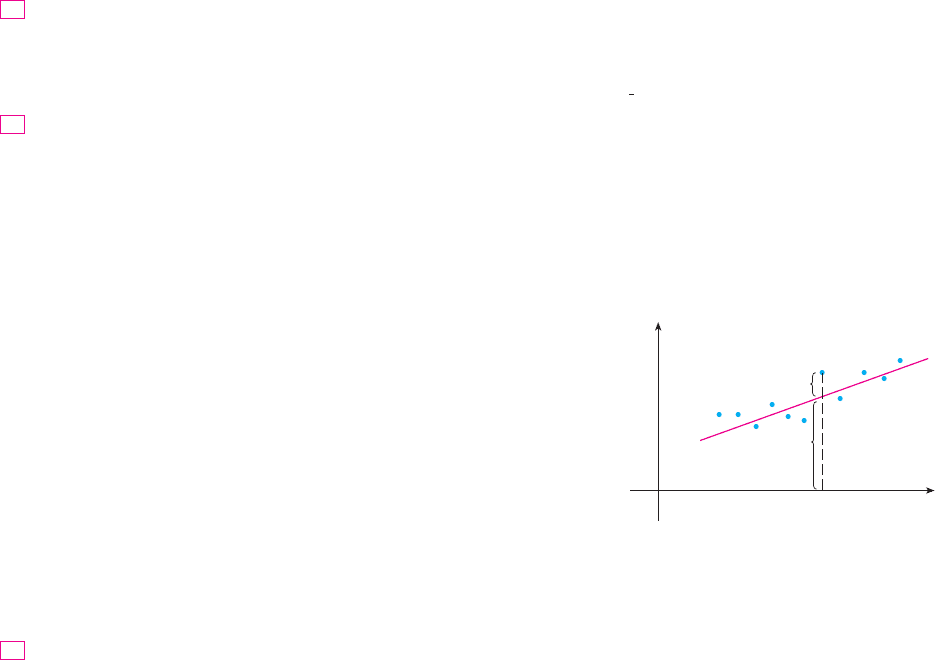
55. Suppose that a scientist has reason to believe that two quan-

tities and are related linearly, that is, , at least

approximately, for some values of and . The scientist

performs an experiment and collects data in the form of points

, , , and then plots these points. The

points don’t lie exactly on a straight line, so the scientist wants

to ﬁnd constants and so that the line “ﬁts” the

points as well as possible. (See the ﬁgure.)

Let be the vertical deviation of the point

from the line. The method of least squares determines

and so as to minimize , the sum of the squares of

these deviations. Show that, according to this method, the line

of best ﬁt is obtained when

Thus the line is found by solving these two equations in the

two unknowns and . (See Section 1.2 for a further discus-

sion and applications of the method of least squares.)

56. Find an equation of the plane that passes through the point

and cuts off the smallest volume in the ﬁrst octant.共1, 2, 3兲

兺

i苷1

⫹ b

兺

i苷1

苷

兺

i苷1

兺

i苷1

⫹ bn 苷

兺

i苷1

冘

i苷1

共x

, y

兲

苷 y

⫺ 共mx

⫹ b兲

(⁄,›)

,y

)

y 苷 mx ⫹ bbm

..., 共x

, y

兲共x

, y

兲共x

, y

兲

y 苷 mx ⫹ byx

Pp ⫹ q ⫹ r 苷 1

rqp

P 苷 2pq ⫹ 2pr ⫹ 2rq

an absolute maximum. But this is not true for functions of two

variables. Show that the function

has exactly one critical point, and that has a local maximum

there that is not an absolute maximum. Then use a computer to

produce a graph with a carefully chosen domain and viewpoint

to see how this is possible.

39. Find the shortest distance from the point to the

plane .

40. Find the point on the plane that is closest to the

point .

Find the points on the cone that are closest to the

point .

42. Find the points on the surface that are closest to

the origin.

Find three positive numbers whose sum is 100 and whose

product is a maximum.

44. Find three positive numbers whose sum is 12 and the sum of

whose squares is as small as possible.

45. Find the maximum volume of a rectangular box that is

inscribed in a sphere of radius .

46. Find the dimensions of the box with volume that has

minimal surface area.

47. Find the volume of the largest rectangular box in the ﬁrst

octant with three faces in the coordinate planes and one

vertex in the plane .

48. Find the dimensions of the rectangular box with largest

volume if the total surface area is given as 64 cm .

49. Find the dimensions of a rectangular box of maximum volume

such that the sum of the lengths of its 12 edges is a constant .

50. The base of an aquarium with given volume is made of slate

and the sides are made of glass. If slate costs ﬁve times as

much (per unit area) as glass, ﬁnd the dimensions of the aquar-

ium that minimize the cost of the materials.

A cardboard box without a lid is to have a volume of

32,000 cm Find the dimensions that minimize the amount

of cardboard used.

52. A rectangular building is being designed to minimize

heat loss. The east and west walls lose heat at a rate of

per day, the north and south walls at a rate of

per day, the ﬂoor at a rate of per day, and

the roof at a rate of per day. Each wall must be at

least 30 m long, the height must be at least 4 m, and the

volume must be exactly .

(a) Find and sketch the domain of the heat loss as a function of

the lengths of the sides.

4000 m

5 units兾m

1 unit兾m

8 units兾m

10 units兾m

51.

x ⫹ 2y ⫹ 3z 苷 6

1000 cm

43.

苷 9 ⫹ xz

共4, 2, 0兲

苷 x

⫹ y

41.

共1, 2, 3兲

x ⫺ y ⫹ z 苷 4

x ⫹ y ⫺ z 苷 1

共2, 1, ⫺1兲

f 共x, y兲苷 3xe

⫺ x

⫺ e

For this project we locate a trash dumpster in order to study its shape and construction. We

then attempt to determine the dimensions of a container of similar design that minimize

construction cost.

1. First locate a trash dumpster in your area. Carefully study and describe all details of its con-

struction, and determine its volume. Include a sketch of the container.

2. While maintaining the general shape and method of construction, determine the dimensions

such a container of the same volume should have in order to minimize the cost of construc-

tion. Use the following assumptions in your analysis:

The sides, back, and front are to be made from 12-gauge (0.1046 inch thick) steel sheets,

which cost $0.70 per square foot (including any required cuts or bends).

The base is to be made from a 10-gauge (0.1345 inch thick) steel sheet, which costs $0.90

per square foot.

Lids cost approximately $50.00 each, regardless of dimensions.

Welding costs approximately $0.18 per foot for material and labor combined.

Give justiﬁcation of any further assumptions or simpliﬁcations made of the details of

construction.

3. Describe how any of your assumptions or simpliﬁcations may affect the ﬁnal result.

4. If you were hired as a consultant on this investigation, what would your conclusions be?

Would you recommend altering the design of the dumpster? If so, describe the savings that

would result.

DESIGNING A DUMPSTER

APPLIED

PROJECT

DISCOVERY PROJECT QUADRATIC APPROXIMATIONS AND CRITICAL POINTS

||||

969

The Taylor polynomial approximation to functions of one variable that we discussed in Chap-

ter 12 can be extended to functions of two or more variables. Here we investigate quadratic

approximations to functions of two variables and use them to give insight into the Second

Derivatives Test for classifying critical points.

In Section 15.4 we discussed the linearization of a function of two variables at a

point :

Recall that the graph of is the tangent plane to the surface at and the

corresponding linear approximation is . The linearization is also called the

ﬁrst-degree Taylor polynomial of at .

1. If has continuous second-order partial derivatives at , then the second-degree Taylor

polynomial of at is

and the approximation is called the quadratic approximation to at .

Verify that has the same ﬁrst- and second-order partial derivatives as at

共a, b兲.fQ

共a, b兲ff 共x, y兲⬇Q共x, y兲

⫹

共a, b兲共x ⫺ a兲

⫹ f

共a, b兲共x ⫺ a兲共y ⫺ b兲 ⫹

共a, b兲共y ⫺ b兲

Q共x, y兲苷 f 共a, b兲 ⫹ f

共a, b兲共x ⫺ a兲 ⫹ f

共a, b兲共y ⫺ b兲

共a, b兲f

Lf 共x, y兲⬇L共x, y兲

共a, b, f 共a, b兲兲z 苷 f 共x, y兲L

L共x, y兲苷 f 共a, b兲 ⫹ f

共a, b兲共x ⫺ a兲 ⫹ f

共a, b兲共y ⫺ b兲

共a, b兲

QUADRATIC APPROXIMATIONS AND CRITICAL POINTS

DISCOVERY

PROJECT

970

||||

CHAPTER 15 PARTIAL DERIVATIVES

2. (a) Find the ﬁrst- and second-degree Taylor polynomials and of

at (0, 0).

;

(b) Graph , , and . Comment on how well and approximate .

3. (a) Find the ﬁrst- and second-degree Taylor polynomials and for at (1, 0).

(b) Compare the values of , , and at (0.9, 0.1).

;

4. In this problem we analyze the behavior of the polynomial

(without using the Second Derivatives Test) by identifying the graph as a paraboloid.

(a) By completing the square, show that if , then

(b) Let . Show that if and , then has a local minimum

at (0, 0).

(d) Show that if , then (0, 0) is a saddle point.

5. (a) Suppose is any function with continuous second-order partial derivatives such that

and (0, 0) is a critical point of . Write an expression for the second-degree

Taylor polynomial, , of at (0, 0).

(b) What can you conclude about from Problem 4?

about ?

f 共x, y兲⬇Q共x, y兲

ff 共0, 0兲苷 0

⬍

D ⬎ 0

fa ⬎ 0D ⬎ 0D 苷 4ac ⫺ b

f 共x, y兲苷 ax

⫹ bxy ⫹ cy

苷 a

冋冉

x ⫹

冊

⫹

冉

4ac ⫺ b

冊

册

a 苷 0

f 共x, y兲苷 ax

⫹ bxy ⫹ cy

fQLQLf

fQL

f 共x, y兲苷 xe

fQLQLf

f 共x, y兲苷 e

⫺x

⫺y

LAGRANGE MULTIPLIERS

In Example 6 in Section 15.7 we maximized a volume function subject to the

constraint , which expressed the side condition that the surface area

was 12 m . In this section we present Lagrange’s method for maximizing or minimizing

a general function subject to a constraint (or side condition) of the form

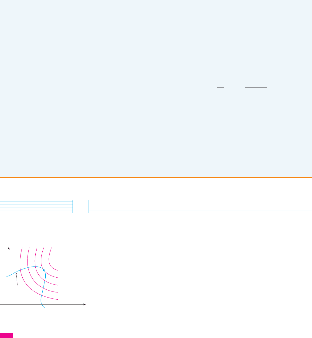
It’s easier to explain the geometric basis of Lagrange’s method for functions of two

variables. So we start by trying to ﬁnd the extreme values of subject to a constraint

of the form . In other words, we seek the extreme values of when the

point is restricted to lie on the level curve . Figure 1 shows this curve

together with several level curves of . These have the equations where ,

, , , . To maximize subject to is to ﬁnd the largest value of such

that the level curve intersects . It appears from Figure 1 that this

happens when these curves just touch each other, that is, when they have a common tan-

gent line. (Otherwise, the value of c could be increased further.) This means that the nor-

mal lines at the point where they touch are identical. So the gradient vectors are

parallel; that is, for some scalar .

This kind of argument also applies to the problem of ﬁnding the extreme values of

subject to the constraint . Thus the point is restricted to lie

on the level surface with equation . Instead of the level curves in Figure 1,

we consider the level surfaces and argue that if the maximum value of

is , then the level surface is tangent to the level surface

and so the corresponding gradient vectors are parallel.t共x, y, z兲苷 k

f 共x, y, z兲苷 cf 共x

, y

, z

兲苷 c

ff 共x, y, z兲苷 c

t共x, y, z兲苷 kS

共x, y, z兲t共x, y, z兲苷 kf 共x, y, z兲

␭

ⵜf 共x

, y

兲苷

␭

ⵜt共x

, y

兲

共x

, y

兲

t共x, y兲苷 kf 共x, y兲苷 c

ct共x, y兲苷 kf 共x, y兲111098

c 苷 7f 共x, y兲苷 c,f

t共x, y兲苷 k共x, y兲

f 共x, y兲t共x, y兲苷 k

f 共x, y兲

t共x, y, z兲苷 k

f 共x, y, z兲

2xz ⫹ 2yz ⫹ xy 苷 12

V 苷 xyz

15.8

f(x,y)=11

f(x,y)=10

f(x,y)=9

f(x,y)=8

f(x,y)=7

g(x,y)=k

FIGURE 1

Visual 15.8 animates Figure 1 for

both level curves and level surfaces.

TEC

This intuitive argument can be made precise as follows. Suppose that a function has

an extreme value at a point on the surface and let be a curve with vector

equation that lies on and passes through . If is the parameter

value corresponding to the point , then . The composite function

represents the values that takes on the curve . Since has an

extreme value at , it follows that has an extreme value at , so . But

if is differentiable, we can use the Chain Rule to write

This shows that the gradient vector is orthogonal to the tangent vector

to every such curve . But we already know from Section 15.6 that the gradient vector

of , , is also orthogonal to for every such curve

(See Equation 15.6.18.)

This means that the gradient vectors and must be parallel.

Therefore, if , there is a number such that

The number in Equation 1 is called a Lagrange multiplier. The procedure based on

Equation 1 is as follows.

METHOD OF LAGRANGE MULTIPLIERS To ﬁnd the maximum and minimum values

of subject to the constraint [assuming that these extreme

values exist and on the surface ]:

(a) Find all values of , , , and such that

and

(b) Evaluate at all the points that result from step (a). The largest of

these values is the maximum value of ; the smallest is the minimum value

of .

If we write the vector equation in terms of its components, then the equa-

tions in step (a) become

This is a system of four equations in the four unknowns , , , and , but it is not neces-

sary to ﬁnd explicit values for .

For functions of two variables the method of Lagrange multipliers is similar to the

method just described. To ﬁnd the extreme values of subject to the constraint

, we look for values of , , and such that

t共x, y兲苷 kandⵜf 共x, y兲苷

␭

ⵜt共x, y兲

␭

yxt共x, y兲苷 k

f 共x, y兲

␭

zyx

t共x, y, z兲苷 kf

苷

␭

苷

␭

苷

␭

ⵜf 苷

␭

ⵜt

共x, y, z兲f

t共x, y, z兲苷 k

ⵜf 共x, y, z兲苷

␭

ⵜt共x, y, z兲

␭

zyx

t共x, y, z兲苷 kⵜt 苷 0

t共x, y, z兲苷 kf 共x, y, z兲

␭

ⵜf 共x

, y

, z

兲苷

␭

ⵜt共x

, y

, z

兲

␭

ⵜt共x

, y

, z

兲苷 0

ⵜt共x

, y

, z

兲ⵜ f 共x

, y

, z

兲

r⬘共t

兲ⵜt共x

, y

, z

兲t

r⬘共t

兲ⵜf 共x

, y

, z

兲

苷 ⵜ f 共x

, y

, z

兲 ⴢ r⬘共t

兲

苷 f

共x

, y

, z

兲x⬘共t

兲 ⫹ f

共x

, y

, z

兲y⬘共t

兲 ⫹ f

共x

, y

, z

兲z⬘共t

兲

0 苷 h⬘共t

兲

h⬘共t

兲苷 0t

h共x

, y

, z

兲

fCfh共t兲苷 f 共x共t兲, y共t兲, z共t兲兲

r共t

兲苷具x

, y

, z

典P

PSr共t兲苷具x共t兲, y共t兲, z共t兲典

CSP共x

, y

, z

兲

SECTION 15.8 LAGRANGE MULTIPLIERS

||||

971

N Lagrange multipliers are named after the

French-Italian mathematician Joseph-Louis

Lagrange (1736–1813). See page 217 for a

biographical sketch of Lagrange.

N In deriving Lagrange’s method we assumed

that . In each of our examples you can

check that at all points where

. See Exercise 21 for what can

go wrong if .ⵜt 苷 0

t共x, y, z兲苷 k

ⵜt 苷 0