Stewart J. Calculus
Подождите немного. Документ загружается.

In general there are four cases for exponents and bases:
1. ( and are constants)
2.
3.
4.
To find , logarithmic differentiation can be used, as in the next
example.
EXAMPLE 4 Differentiate .
SOLUTION 1 Using logarithmic differentiation, we have
SOLUTION 2 Another method is to write :
(as in Solution 1) M
GENERAL LOGARIT H M I C F U N C TI O N S
If and , then is a one-to-one function. Its inverse function is called
the logarithmic function with base a and is denoted by . Thus
In particular, we see that
The cancellation equations for the inverse functions and are
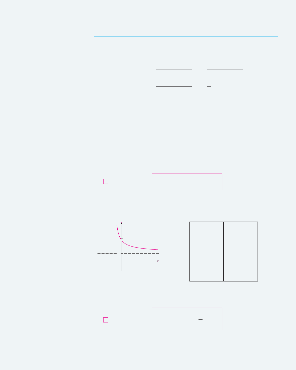
Figure 9 shows the case where . (The most important logarithmic functions have
base .) The fact that is a very rapidly increasing function for is
reflected in the fact that is a very slowly increasing function for .
x % 1y ! log
a
x
x % 0y ! a
x
a % 1
a % 1
log
a
!a
x
" ! xanda
log
a
x
! x
a
x
log
a
x
log
e
x ! ln x
log
a
x ! y &? a
y
! x
5
log
a
f !x" ! a
x
a " 1a % 0
! x
s
x
)
2 & ln x
2
s
x
*
d
dx
(
x
s
x
)
!
d
dx
(
e
s
x
ln x
)
! e
s
x
ln x
d
dx
(
s
x
ln x
)
x
s
x
! !e
ln x
"
s
x
y' ! y
)
1
s
x
&
ln x
2
s
x
*
! x
s
x
)
2 & ln x
2
s
x
*
y'
y
!
s
x
!
1
x
& !ln x"
1
2
s
x
ln y ! ln x
s
x
!
s
x
ln x
y ! x
s
x
V
!d#dx"' f !x"(
t!x"
d
dx
'a
t!x"
( ! a
t!x"
!ln a"t'!x"
d
dx
' f !x"(
b
! b' f !x"(
b!1
f '!x"
ba
d
dx
!a
b
" ! 0
442
|| ||
CHAPTER 7 INVERSE FUNCTIONS
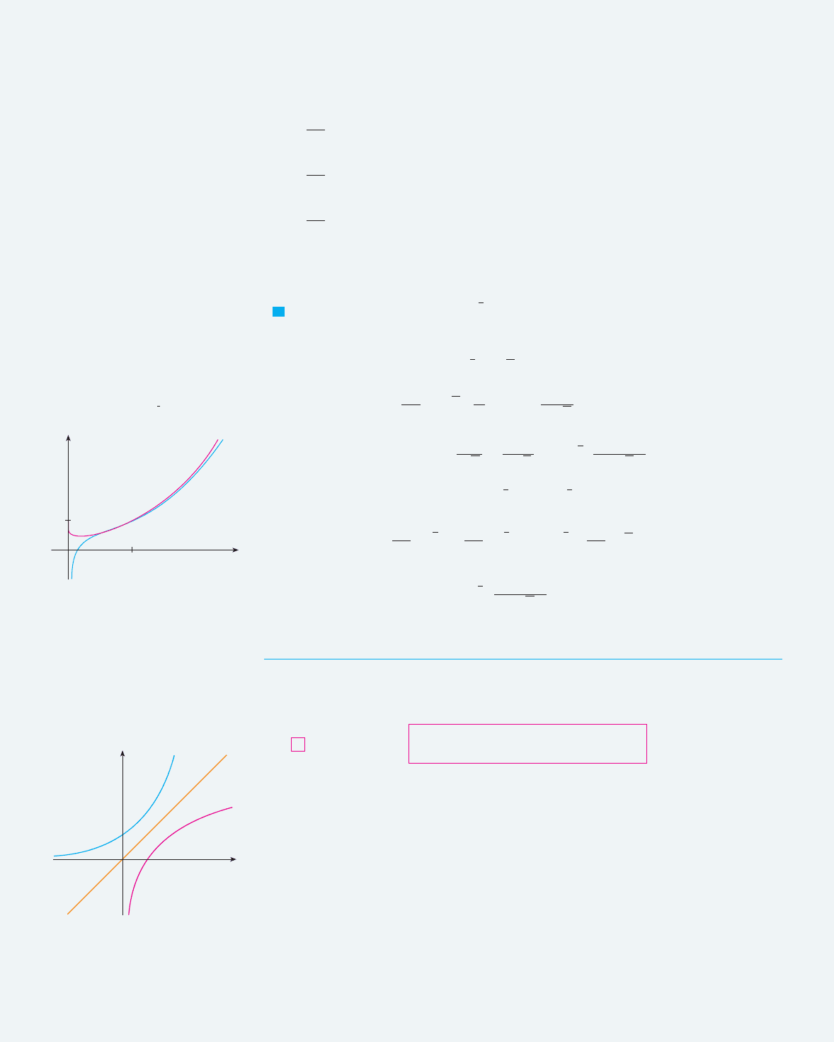
N Figure 8 illustrates Example 4 by showing
the graphs of and its derivative.
f !x" ! x
s
x
*
F I G U R E 8
1
1
f
fª
x
0
y
0
y=x
y=a®,a>1
y=log
a
x, a>1
F I G U R E 9
y
x

Figure 10 shows the graphs of with various values of the base . Since
, the graphs of all logarithmic functions pass through the point .
The laws of logarithms are similar to those for the natural logarithm and can be deduced
from the laws of exponents (see Exercise 65).
The following formula shows that logarithms with any base can be expressed in terms
of the natural logarithm.
CHANGE OF BASE FORMULA For any positive number , we have
PROOF Let . Then, from (5), we have . Taking natural logarithms of both
sides of this equation, we get . Therefore
M
Scientific calculators have a key for natural logarithms, so Formula 6 enables us to use
a calculator to compute a logarithm with any base (as shown in the following example).
Similarly, Formula 6 allows us to graph any logarithmic function on a graphing calculator
or computer (see Exercises 14 –16).
EXAMPLE 5 Evaluate correct to six decimal places.
SOLUTION Formula 6 gives
M
Formula 6 enables us to differentiate any logarithmic function. Since is a constant,
we can differentiate as follows:
EXAMPLE 6 Using Formula 7 and the Chain Rule, we get
M
From Formula 7 we see one of the main reasons that natural logarithms (logarithms
with base ) are used in calculus: The differentiation formula is simplest when
because .ln e ! 1
a ! ee
!
cos x
!2 & sin x" ln 10
d
dx
log
10
!2 & sin x" !
1
!2 & sin x" ln 10
d
dx
!2 & sin x"
d
dx
!log
a
x" !
1
x ln a
7
d
dx
!log
a
x" !
d
dx
)
ln x
ln a
*
!
1
ln a
d
dx
!ln x" !
1
x ln a
ln a
log
8
5 !
ln 5
ln 8
+ 0.773976
log
8
5
y !
ln x
ln a
y ln a ! ln x
a
y
! xy ! log
a
x
log
a
x !
ln x
ln a
!a " 1"a
6
!1, 0"log
a
1 ! 0
ay ! log
a
x
SECTION 7.4* GENERAL LOGARITHMIC AND EXPONENTIAL FUNCTIONS
|| ||
443
F I G U R E 1 0
0
y
1
x
1
y=log£x
y=log™x
y=log∞x
y=log¡¸x
N NOTATION FOR LOGARITHMS
Most textbooks in calculus and the sciences, as
well as calculators, use the notation for the
natural logarithm and for the “common
logarithm,” . In the more advanced mathe-
matical and scientific literature and in computer
languages, however, the notation usually
denotes the natural logarithm.
log x
log
10
x
log x
ln x
THE NUMBER
e
AS A LIMIT
We have shown that if , then . Thus . We now use this fact
to express the number as a limit.
From the definition of a derivative as a limit, we have
Because , we have
Then, by Theorem 2.5.8 and the continuity of the exponential function, we have
Formula 8 is illustrated by the graph of the function in Figure 11 and a
table of values for small values of .
If we put in Formula 8, then as and so an alternative expression
for is
e ! lim
n l !
!
1 "
1
n
"
n
9
e
x l 0
"
n l !n ! 1#x
F I G U R E 1 1
2
3
y=(1+x)!?®
1
0
y
x
x
y ! $1 " x%
1#x
e ! lim
x l 0
$1 " x%
1#x
8
e ! e
1
! e
lim
x
l
0
ln$1"x%
1#x
! lim
x
l
0
e
ln$1"x%
1#x
! lim
x
l
0
$1 " x%
1#x
lim
x
l
0
ln$1 " x%
1#x
! 1
f #$1% ! 1
! lim
x l 0
ln$1 " x%
1#x
! lim
x l 0
ln$1 " x% $ ln 1
x
! lim
x l 0
1
x
ln$1 " x%
f #$1% ! lim
h l 0
f $1 " h% $ f $1%
h
! lim
x l 0
f $1 " x% $ f $1%
x
e
f #$1% ! 1f #$x% ! 1#xf $x% ! ln x
444
|| ||
CHAPTER 7 INVERSE FUNCTIONS
x
0.1 2.59374246
0.01 2.70481383
0.001 2.71692393
0.0001 2.71814593
0.00001 2.71826824
0.000001 2.71828047
0.0000001 2.71828169
0.00000001 2.71828181
(1 " x)
1/x
SECTION 7.4* GENERAL LOGARITHMIC AND EXPONENTIAL FUNCTIONS
|| ||
445
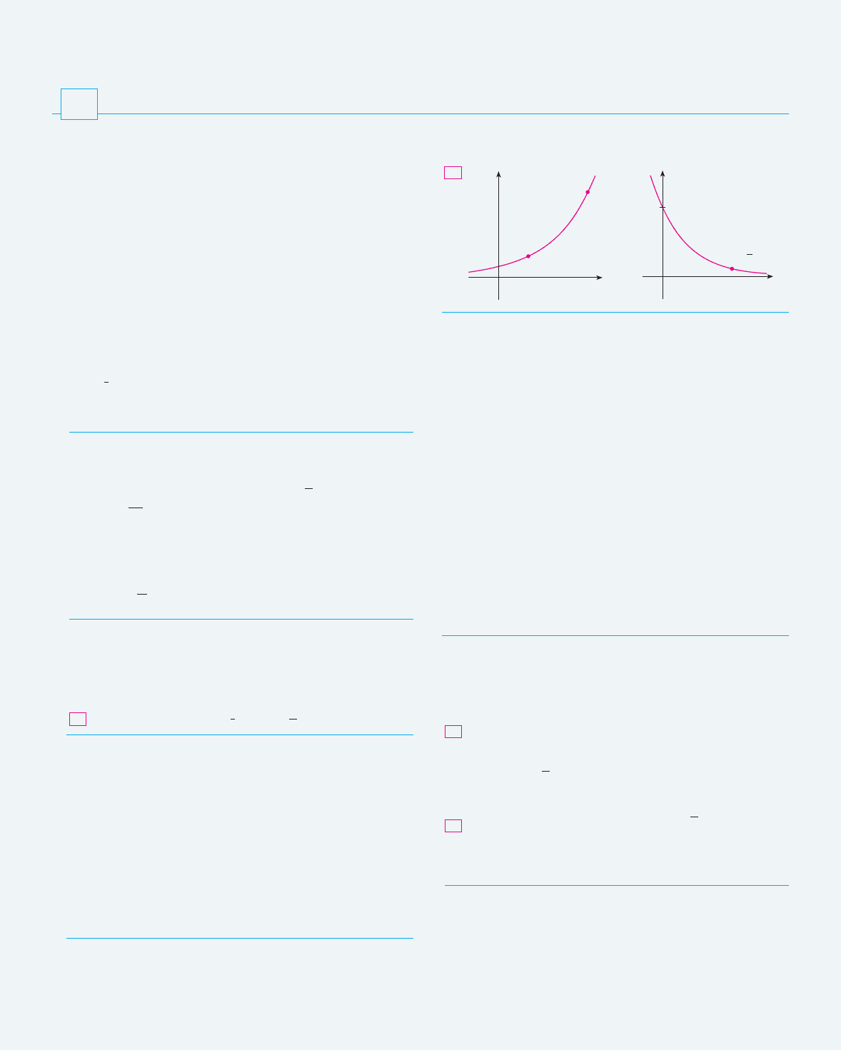
17–18 Find the exponential function whose graph is
given.
18.
19. (a) Show that if the graphs of and are
drawn on a coordinate grid where the unit of measure-
ment is 1 inch, then at a distance 2 ft to the right of the
origin the height of the graph of is 48 ft but the height
of the graph of is about 265 mi.
(b) Suppose that the graph of is drawn on a coor-
dinate grid where the unit of measurement is an inch.
How many miles to the right of the origin do we have to
move before the height of the curve reaches ft?
;
20. Compare the rates of growth of the functions and
by graphing both functions in several viewing rect-
angles. Find all points of intersection of the graphs correct to
one decimal place.
21–24 Find the limit.
21. 22.
23. 24.
25– 42 Differentiate the function.
25. 26.
27. 28.
30.
31. 32.
33. 34.
35. 36.
38.
39. 40.
41. 42.
43. Find an equation of the tangent line to the curve at
the point .
$1, 10%
y ! 10
x
y ! $ln x%
cos x
y ! $tan x%
1#x
y ! $sin x%
ln x
y ! $cos x%
x
y !
s
x
x
y ! x
sin x
37.
y ! x
cos x
y ! x
x
y ! log
2
$e
$x
cos
%
x%y ! 2x log
10
s
x
f $x% ! log
5
$xe
x
%f $x% ! log
2
$1 $ 3x%
y ! 2
3
x
2
f$u% ! $2
u
" 2
$u
%
10
29.
y ! 10
tan
&
y ! 5
$1#x
t$x% ! x
4
4
x
h$t% ! t
3
$ 3
t
lim
x
l
3
"
log
10
$x
2
$ 5x " 6%lim
t
l
!
2
$t
2
lim
x
l
$!
$1.001%
x
lim
x l !
$1.001%
x
t$x% ! 5
x
f $x% ! x
5
3
y ! log
2
x
t
f
t$x% ! 2
x
f $x% ! x
2
”2, ’
2
9
0
2
y
x
0
(1,6)
(3,24)
y
x
17.
f $x% ! Ca
x
1. (a) Write an equation that defines when is a positive
number and is a real number.
(b) What is the domain of the function ?
(c) If , what is the range of this function?
(d) Sketch the general shape of the graph of the exponential
function for each of the following cases.
(i) (ii) (iii)
2. (a) If is a positive number and , how is
defined?
(b) What is the domain of the function ?
(c) What is the range of this function?
(d) If , sketch the general shapes of the graphs of
and with a common set of axes.
3–6 Write the expression as a power of .
3. 4.
5. 6.
7–10 Evaluate the expression.
7. (a) (b)
8. (b)
9. (a)
(b)
10. (a) (b)
;
11–12 Graph the given functions on a common screen. How are
these graphs related?
11. , , ,
, , ,
13. Use Formula 6 to evaluate each logarithm correct to six deci-
mal places.
(a) (b) (c)
;
14 –16 Use Formula 6 to graph the given functions on a common
screen. How are these graphs related?
14. , , ,
15. , , ,
16. , , , y ! 10
x
y ! e
x
y ! log
10
xy ! ln x
y ! log
50
xy ! log
10
xy ! ln xy ! log
1.5
x
y ! log
8
xy ! log
6
xy ! log
4
xy ! log
2
x
log
2
%
log
6
13.54log
12
e
y !
(
1
10
)
x
y !
(
1
3
)
x
y ! 10
x
y ! 3
x
12.
y ! 20
x
y ! 5
x
y ! e
x
y ! 2
x
10
$log
10
4"log
10
7%
log
a
1
a
log
3
100 $ log
3
18 $ log
3
50
log
2
6 $ log
2
15 " log
2
20
log
8
320 $ log
8
5log
10
s
10
log
3
1
27
log
5
125
x
cos x
$cos x%
x
10
x
2
5
s
7
e
y ! a
x
y ! log
a
x
a ' 1
f $x% ! log
a
x
log
a
xa " 1a
0
(
a
(
1a ! 1a ' 1
a " 1
f $x% ! a
x
x
aa
x
E X E R C I S E S
7.4*

(b) If and , find the rate of change of
intensity with respect to depth at a depth of 20 m.
(c) Using the values from part (b), find the average light
intensity between the surface and a depth of 20 m.
;
61. The flash unit on a camera operates by storing charge on a
capacitor and releasing it suddenly when the flash is set off.
The following data describe the charge remaining on the
capacitor (measured in microcoulombs, )C) at time (mea-
sured in seconds).
(a) Use a graphing calculator or computer to find an expo-
nential model for the charge.
(b) The derivative represents the electric current (mea-
sured in microamperes, )A) flowing from the capacitor to
the flash bulb. Use part (a) to estimate the current when
s. Compare with the result of Example 2 in
Section 2.1.
;
62. The table gives the US population from 1790 to 1860.
(a) Use a graphing calculator or computer to fit an exponen-
tial function to the data. Graph the data points and the
exponential model. How good is the fit?
(b) Estimate the rates of population growth in 1800 and 1850
by averaging slopes of secant lines.
(c) Use the exponential model in part (a) to estimate the rates
of growth in 1800 and 1850. Compare these estimates
with the ones in part (b).
(d) Use the exponential model to predict the population in
1870. Compare with the actual population of 38,558,000.
Can you explain the discrepancy?
63. Prove the second law of exponents [see (3)].
64. Prove the fourth law of exponents [see (3)].
65. Deduce the following laws of logarithms from (3):
(a)
(b)
(c)
66. Show that for any .
x ' 0lim
n l !
!
1 "
x
n
"
n
! e
x
log
a
$x
y
% ! y log
a
x
log
a
$x#y% ! log
a
x $ log
a
y
log
a
$xy% ! log
a
x " log
a
y
t ! 0.04
Q#$t%
t
Q
a ! 0.38I
0
! 8
;
44. If , find . Check that your answer is reason-
able by comparing the graphs of and .
45–50 Evaluate the integral.
46.
47. 48.
50.
51. Find the area of the region bounded by the curves ,
, , and .
52. The region under the curve from to is
rotated about the -axis. Find the volume of the resulting
solid.
;
53. Use a graph to find the root of the equation cor-
rect to one decimal place. Then use this estimate as the initial
approximation in Newton’s method to find the root correct to
six decimal places.
Find if .
55. Find the inverse function of .
56. Calculate .
57. The geologist C. F. Richter defined the magnitude of an
earthquake to be , where is the intensity of the
quake (measured by the amplitude of a seismograph 100 km
from the epicenter) and is the intensity of a “standard”
earthquake (where the amplitude is only 1 micron cm).
The 1989 Loma Prieta earthquake that shook San Francisco
had a magnitude of 7.1 on the Richter scale. The 1906 San
Francisco earthquake was 16 times as intense. What was its
magnitude on the Richter scale?
58. A sound so faint that it can just be heard has intensity
watt#m at a frequency of 1000 hertz (Hz). The
loudness, in decibels (dB), of a sound with intensity is then
defined to be . Amplified rock music is
measured at 120 dB, whereas the noise from a motor-driven
lawn mower is measured at 106 dB. Find the ratio of the
intensity of the rock music to that of the mower.
59. Referring to Exercise 58, find the rate of change of the loud-
ness with respect to the intensity when the sound is measured
at 50 dB (the level of ordinary conversation).
60. According to the Beer-Lambert Law, the light intensity at a
depth of meters below the surface of the ocean is
, where is the light intensity at the surface and
is a constant such that .
(a) Express the rate of change of with respect to in
terms of .
I$x%
xI$x%
0
(
a
(
1
aI
0
I$x% ! I
0
a
x
x
L ! 10 log
10
$I#I
0
%
I
2
I
0
! 10
$12
! 10
$4
S
Ilog
10
$I#S %
lim
x l !
x
$ln x
f $x% ! log
10
!
1 "
1
x
"
x
y
! y
x
y#
54.
2
x
! 1 " 3
$x
x
x ! 1x ! 0y ! 10
$x
x ! 1x ! $1y ! 5
x
y ! 2
x
y
2
x
2
x
" 1
dx
y
3
sin
&
cos
&
d
&
49.
y
x2
x
2
dx
y
log
10
x
x
dx
y
$x
5
" 5
x
% dx
y
2
1
10
t
dt
45.
f #f
f #$x%f $x% ! x
cos x
446
|| ||
CHAPTER 7 INVERSE FUNCTIONS
t 0.00 0.02 0.04 0.06 0.08 0.10
Q 100.00 81.87 67.03 54.88 44.93 36.76
Year Population Year Population
1790 3,929,000 1830 12,861,000
1800 5,308,000 1840 17,063,000
1810 7,240,000 1850 23,192,000
1820 9,639,000 1860 31,443,000

EXP ONEN TIAL GROW TH A ND D EC AY
In many natural phenomena, quantities grow or decay at a rate proportional to their size.
For instance, if is the number of individuals in a population of animals or bacte-
ria at time , then it seems reasonable to expect that the rate of growth is proportion-
al to the population ; that is, for some constant . Indeed, under ideal
conditions (unlimited environment, adequate nutrition, immunity to disease) the mathe-
matical model given by the equation predicts what actually happens fairly
accurately. Another example occurs in nuclear physics where the mass of a radioactive
substance decays at a rate proportional to the mass. In chemistry, the rate of a unimolecu-
lar first-order reaction is proportional to the concentration of the substance. In finance, the
value of a savings account with continuously compounded interest increases at a rate pro-
portional to that value.
In general, if is the value of a quantity at time and if the rate of change of with
respect to is proportional to its size at any time, then
where is a constant. Equation 1 is sometimes called the law of natural growth (if )
or the law of natural decay (if ). It is called a differential equation because it
involves an unknown function and its derivative .
It’s not hard to think of a solution of Equation 1. This equation asks us to find a function
whose derivative is a constant multiple of itself. We have met such functions in this chap-
ter. Any exponential function of the form , where is a constant, satisfies
We will see in Section 10.4 that any function that satisfies must be of the form
. To see the significance of the constant , we observe that
Therefore is the initial value of the function.
THEOREM The only solutions of the differential equation are the
exponential functions
POPULATION GROW T H
What is the significance of the proportionality constant k? In the context of population
growth, where is the size of a population at time , we can write
1
P
dP
dt
! kor
dP
dt
! kP
3
tP$t%
y$t% ! y$0%e
kt
dy#dt ! ky
2
C
y$0% ! Ce
k! 0
! C
Cy ! Ce
kt
dy#dt ! ky
y#$t% ! C$ke
kt
% ! k$Ce
kt
% ! ky$t%
Cy$t% ! Ce
kt
dy#dty
k
(
0
k ' 0k
dy
dt
! ky
1
y$t%t
ytyy$t%
f #$t% ! k f $t%
kf #$t% ! kf $t%f $t%
f #$t%t
y ! f $t%
7.5
SECTION 7.5 EXPONENTIAL GROWTH AND DECAY
|| ||
447

The quantity
is the growth rate divided by the population size; it is called the relative growth rate.
According to (3), instead of saying “the growth rate is proportional to population size” we
could say “the relative growth rate is constant.” Then (2) says that a population with con-
stant relative growth rate must grow exponentially. Notice that the relative growth rate k
appears as the coefficient of t in the exponential function . For instance, if
and t is measured in years, then the relative growth rate is and the population
grows at a relative rate of 2% per year. If the population at time 0 is , then the expres-
sion for the population is
EXAMPLE 1 Use the fact that the world population was 2560 million in 1950 and
3040 million in 1960 to model the population of the world in the second half of the 20th
century. (Assume that the growth rate is proportional to the population size.) What is the
relative growth rate? Use the model to estimate the world population in 1993 and to
predict the population in the year 2020.
SOLUTION We measure the time t in years and let t ! 0 in the year 1950. We measure the
population in millions of people. Then and Since we
are assuming that , Theorem 2 gives
The relative growth rate is about 1.7% per year and the model is
We estimate that the world population in 1993 was
The model predicts that the population in 2020 will be
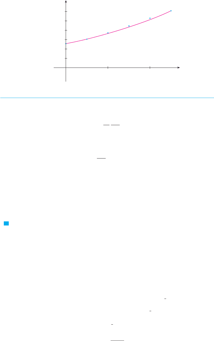
The graph in Figure 1 shows that the model is fairly accurate to the end of the 20th cen-
tury (the dots represent the actual population), so the estimate for 1993 is quite reliable.
But the prediction for 2020 is riskier.
P$70% ! 2560e
0.017185$70%
& 8524 million
P$43% ! 2560e
0.017185$43%
& 5360 million
P$t% ! 2560e
0.017185t
k !
1
10
ln
3040
2560
& 0.017185
P$10% ! 2560e
10k
! 3040
P$t% ! P$0%e
kt
! 2560e
kt
dP#dt ! kP
P$10) ! 3040.P$0% ! 2560P$t%
V
P$t% ! P
0
e
0.02t
P
0
k ! 0.02
dP
dt
! 0.02P
Ce
kt
1
P
dP
dt
448
|| ||
CHAPTER 7 INVERSE FUNCTIONS
M
RADIOACT I V E D E C AY
Radioactive substances decay by spontaneously emitting radiation. If is the mass
remaining from an initial mass of the substance after time t, then the relative decay rate
has been found experimentally to be constant. (Since is negative, the relative decay
rate is positive.) It follows that
where k is a negative constant. In other words, radioactive substances decay at a rate pro-
portional to the remaining mass. This means that we can use (2) to show that the mass
decays exponentially:
Physicists express the rate of decay in terms of half-life, the time required for half of
any given quantity to decay.
EXAMPLE 2 The half-life of radium-226 is 1590 years.
(a) A sample of radium-226 has a mass of 100 mg. Find a formula for the mass of the
sample that remains after years.
(b) Find the mass after 1000 years correct to the nearest milligram.
(c) When will the mass be reduced to 30 mg?
SOLUTION
(a) Let be the mass of radium-226 (in milligrams) that remains after years. Then
and , so (2) gives
In order to determine the value of , we use the fact that . Thus
and
Therefore m$t% ! 100e
$$ln 2%t#1590
k ! $
ln 2
1590
1590k ! ln
1
2
! $ln 2
e
1590k
!
1
2
so100e
1590k
! 50
y$1590% !
1
2
$100%k
m$t% ! m$0%e
kt
! 100e
kt
y$0% ! 100dm#dt ! km
tm$t%
t
V
m$t% ! m
0
e
kt
dm
dt
! km
dm#dt
$
1
m
dm
dt
m
0
m$t%
F I G U R E 1
A model for world population growth
in the second half of the 20th century
6000
P
t
20
40
Years since 1950
Population
(in millions)
P=2560e
0.017185t
SECTION 7.5 EXPONENTIAL GROWTH AND DECAY
|| ||
449
We could use the fact that to write the expression for in the alternative
form
(b) The mass after 1000 years is
(c) We want to find the value of such that , that is,
We solve this equation for by taking the natural logarithm of both sides:
Thus M
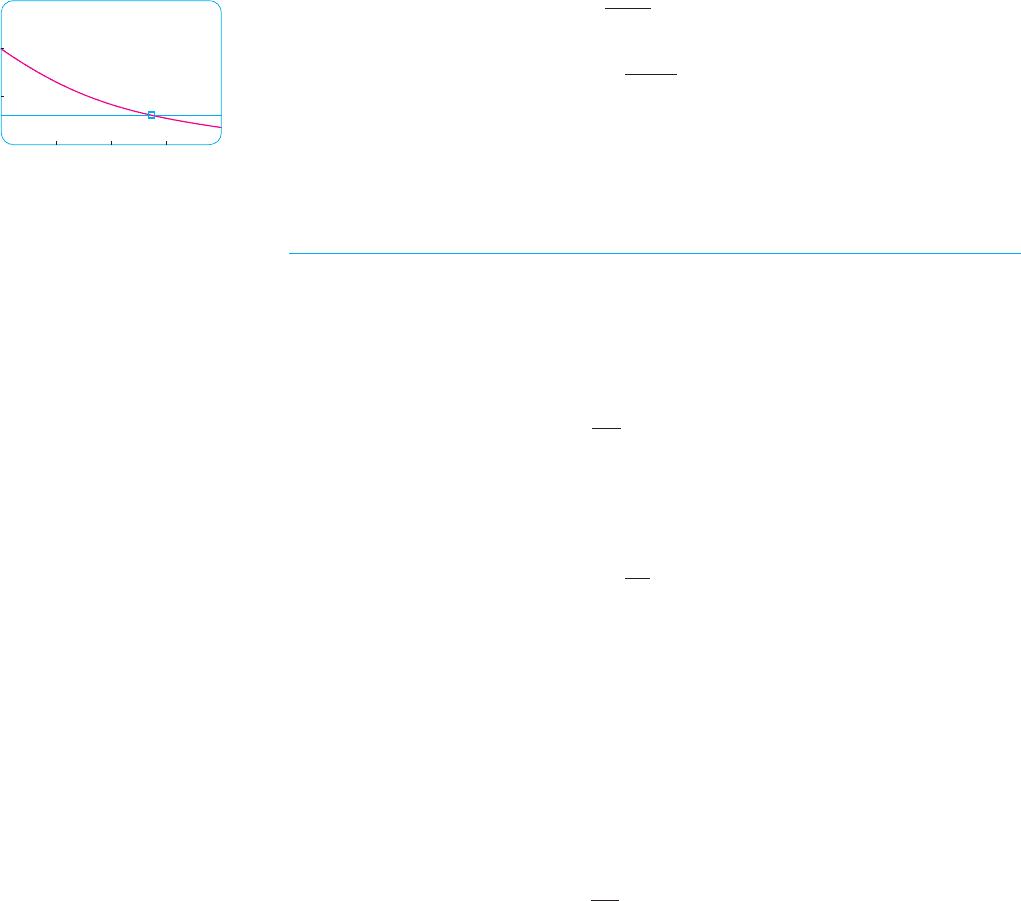
As a check on our work in Example 2, we use a graphing device to draw the graph of
in Figure 2 together with the horizontal line . These curves intersect when
, and this agrees with the answer to part (c).
NEWTON ’ S LAW OF COOLING
Newton’s Law of Cooling states that the rate of cooling of an object is proportional to
the temperature difference between the object and its surroundings, provided that this
difference is not too large. (This law also applies to warming.) If we let be the tem-
perature of the object at time and be the temperature of the surroundings, then we
can formulate Newton’s Law of Cooling as a differential equation:
where is a constant. This equation is not quite the same as Equation 1, so we make
the change of variable . Because is constant, we have
and so the equation becomes
We can then use (2) to find an expression for , from which we can find .
EXAMPLE 3 A bottle of soda pop at room temperature ( F) is placed in a refrigerator
where the temperature is F. After half an hour the soda pop has cooled to F.
(a) What is the temperature of the soda pop after another half hour?
(b) How long does it take for the soda pop to cool to F?
SOLUTION
(a) Let be the temperature of the soda after minutes. The surrounding temperature
is , so Newton’s Law of Cooling states that
dT
dt
! k$T $ 44)
T
s
! 44* F
tT$t%
50*
61*44*
72*
Ty
dy
dt
! ky
y#$t% ! T#$t%T
s
y$t% ! T$t% $ T
s
k
dT
dt
! k$T $ T
s
%
T
s
t
T$t%
t & 2800
m ! 30m$t%
t ! $1590
ln 0.3
ln 2
& 2762 years
$
ln 2
1590
t ! ln 0.3
t
e
$$ln 2%t#1590
! 0.3or100e
$$ln 2%t#1590
! 30
m$t% ! 30t
m$1000% ! 100e
$$ln 2%1000#1590
& 65 mg
m$t% ! 100 + 2
$t#1590
m$t%e
ln 2
! 2
450
|| ||
CHAPTER 7 INVERSE FUNCTIONS
m=30
0
4000
150
m=100e
_(ln2)t/1590
F I G U R E 2
If we let , then , so satisfies
and by (2) we have
We are given that , so and
Taking logarithms, we have
Thus
So after another half hour the pop has cooled to about F.
(b) We have when
The pop cools to F after about 1 hour 33 minutes. M
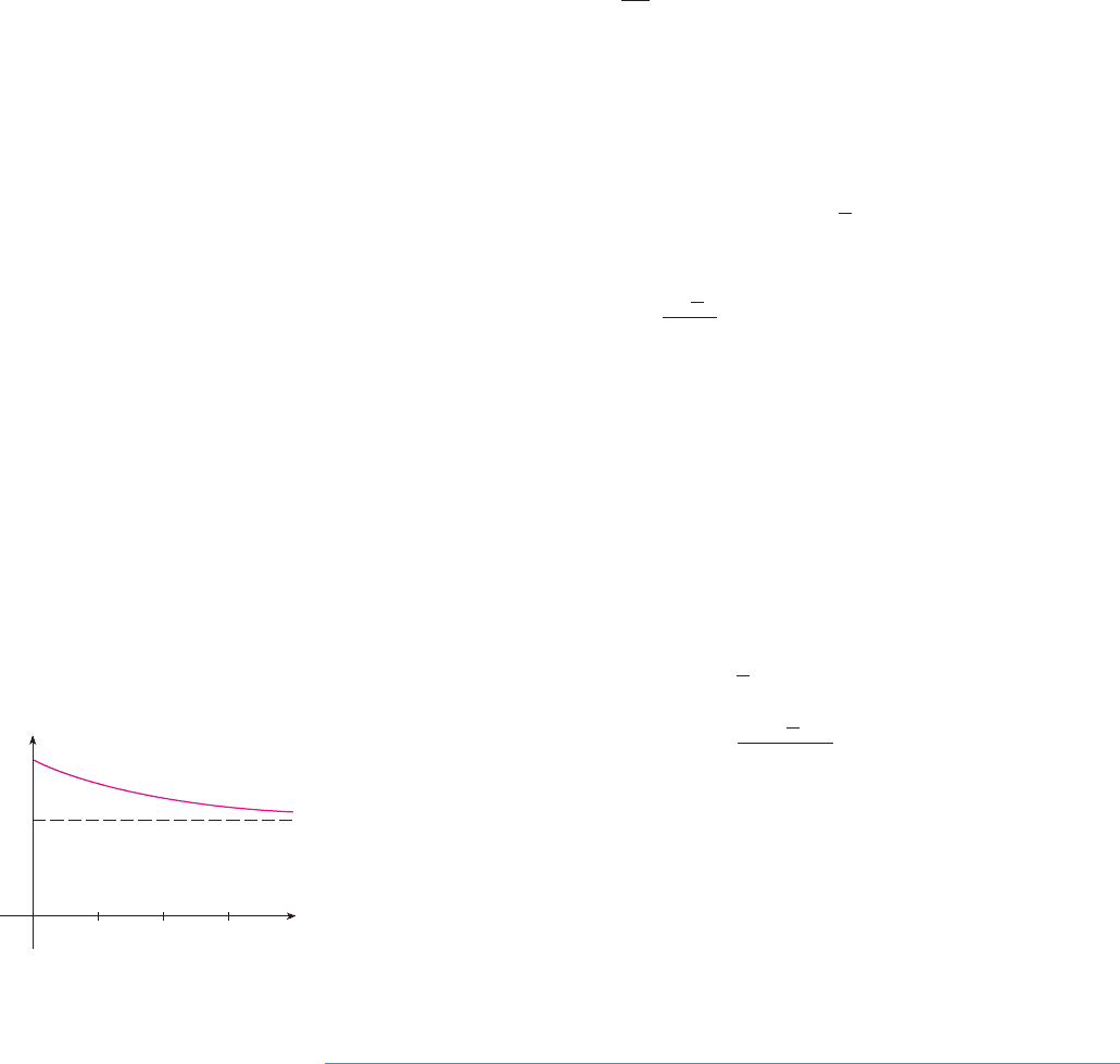
Notice that in Example 3, we have
which is to be expected. The graph of the temperature function is shown in Figure 3.
CONTINUOUS LY COMPOU N D E D I N T E RE S T
EXAMPLE 4 If $1000 is invested at 6% interest, compounded annually, then after
1 year the investment is worth , after 2 years it’s worth
, and after years it’s worth . In general,
if an amount is invested at an interest rate in this example), then after
years it’s worth . Usually, however, interest is compounded more frequently,
say, times a year. Then in each compounding period the interest rate is and there r#nn
A
0
$1 " r%
t
t
$r ! 0.06rA
0
$1000$1.06%
t
t$'1000$1.06%(1.06 ! $1123.60
$1000$1.06% ! $1060
lim
t
l
!
T$t% ! lim
t
l
!
$44 " 28e
$0.01663t
% ! 44 " 28 ! 0 ! 44
50*
t !
ln
(
6
28
)
$0.01663
& 92.6
e
$0.01663t
!
6
28
44 " 28e
$0.01663t
! 50
T$t% ! 50
54*
T$60% ! 44 " 28e
$0.01663$60%
& 54.3
T$t% ! 44 " 28e
$0.01663t
y$t% ! 28e
$0.01663t
k !
ln
(
17
28
)
30
& $0.01663
e
30k
!
17
28
28e
30k
! 17
y$30% ! 61 $ 44 ! 17T$30% ! 61
y$t% ! y$0%e
kt
! 28e
kt
y$0% ! 28
dy
dt
! ky
yy$0% ! T$0% $ 44 ! 72 $ 44 ! 28y ! T $ 44
SECTION 7.5 EXPONENTIAL GROWTH AND DECAY
|| ||
451
F I G U R E 3
72
T
t
60
0
30 90
44