Teodorescu P.P. Mechanical Systems, Classical Models Volume I: Particle Mechanics

Подождите немного. Документ загружается.

MECHANICAL SYSTEMS, CLASSICAL MODELS

472

where we have introduced the apparent potential

()Ur and the constant of energy h ;

hence

d(1 / )

() ()

θθ θ

ϕρ ρ ϕρ

=± =

∫∫

∓ ,

[]

() ()rUrh

ϕ =+

(8.1.6'')

the trajectory in polar co-ordinates being thus specified. The two first integrals used

above allow also to put in evidence the motion of the particle along the trajectory,

establishing its parametric equations in the form

()dtt r

ϑϑ=+

∫

()

ϕρ

=±

∫

(8.1.6''')

If the potential is of the form

() /

Ur k r

, constk

, s

∈

 , then the above

integrals may be expressed by elementary functions only if

2s =− (harmonic

oscillator),

1s =− , 1s = (Keplerian motion) and 2s

; if

6, 4, 3,4, 6s

−−

, then

these integrals may be expressed by means of elliptic functions.

The sign before the radical is determined by the sign of the initial velocity

()rrt=, as long as () 0rϕ > . If () 0rϕ

, it results that

= , so that the

velocity is normal to the radius vector at the initial moment; the motion along the radius

vector takes place as this radius would be fixed, the force which acts upon the particle

being

F . If this apparent force is positive (repulsive force), then r is increasing and

takes the sign +; otherwise, one takes the sign –. In particular, let us suppose that

0F =

at the initial moment; in this case, the particle remains immovable for an

observer on the radius vector, because the particle moves along this radius as if it would

be fixed, the particle being launched without initial velocity at a point in which the

apparent force vanishes. Hence, the trajectory is a circle of radius

r , the motion being

uniform (because the areal velocity is constant).

To have a circular trajectory, it is necessary that

/2απ

± (the velocity be

normal to the radius vector at the initial moment, so that

Crv=±

) and

() / 0Fr mC r+=

. If

(circular motion) and

θθ



(uniform motion),

then – during the motion – the equation (8.1.4) is identically verified; the initial

conditions being fulfilled, the theorem of uniqueness ensures the searched solution. The

velocity at the initial moment has thus the modulus

()Fr r

−

;

(8.1.7)

hence, at the initial moment, the force

F must be of attraction (

() 0Fr < ).

The relation (8.1.4) may be written also in the form

(

)

d1 1

r θ

⎡

⎤

=− +

⎢

⎥

⎣

⎦

;

(8.1.8)

Dynamics of the particle in a field of elastic forces

473

we obtain thus Binet’s formula, which allows to solve the inverse problem: to determine

the central force which, applied upon a given particle, imparts a plane trajectory to it,

after the law of areas with respect to a fixed pole. Taking into account the equation

(8.1.4') of the trajectory, we can write

[]

() ()

Fff

θθ

′′

=− +

(8.1.8')

too, where

f θ

′′

≡∂ ∂ . If beforehand a form of F is not imposed, that one has a

certain non-determination, taking into account the equation of the trajectory (the

equation which links

r to θ ); eliminating θ , one obtains ()FFr

, form used the

most times.

For instance, in case of trajectories to which corresponds the equation

cos

rakbθ=+, ,, constabk

(8.1.9)

choosing the fixed point as origin, we get

(

)

(1)

() ( 2)

kab

Fr k b

+−

⎡

⎤

=− + +

⎢

⎥

⎣

⎦

;

(8.1.9')

in particular, these trajectories may be conics with the pole at the focus (

1k =− ) or at

the centre (

1k = ), Pascal limaçons ( 2k

, 0b

), lemniscates etc.

1.1.2 Qualitative study of orbits. Bertrand’s theorem

Usually, the trajectory of a particle in a central field of forces is called orbit (even if

it is not a closed curve). The relations (8.1.6')-(8.1.6''') determine the orbit and the

motion on it only if

r

and

are real quantities, hence if () 0rϕ ≥ ; the apparent

potential must verify the condition

() 0Ur h

≥

, which determines the domain of

variation of

r , corresponding to the motion of the particle; the solutions of the equation

() 0Ur h

(8.1.10)

specify the frontier of the domain. From (8.1.6') one may see that the radial velocity

vanishes on the frontier (

 ), the angular velocity being non-zero ( 0θ ≠



); if

we would have

0θ =



at a point other than the origin, then the first integral of areas

would lead to

0C =

, that is to a rectilinear trajectory; hence, at the respective points

the velocity is normal to the radius vector. On the frontier,

()rt changes of sign, the

respective point corresponding to a relative extremum for

()rt . The relation (8.1.2)

shows that

()tθ



has a constant sign, so that ()tθ is a monotone function; the integrals

(8.1.6''), (8.1.6''') must be calculated on intervals of monotony, the sign being

chosen correspondingly. Let

min

r and

max

r be the extreme values which may be taken

r ; the corresponding points on the orbit are called apsides. In this case,

MECHANICAL SYSTEMS, CLASSICAL MODELS

474

max

min

0 rrr≤≤≤. The roots of the equation (8.1.10) may be graphically

determined, taking into consideration the intersection of the apparent potential

()UUr= with the straight line Uh

− ; the domain of variation of r corresponds to

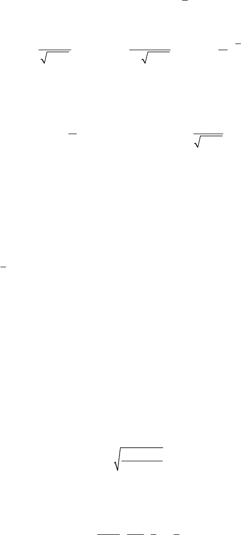
()Ur h≥− (Fig.8.2).

Figure 8.2. Diagram ()Ur vs

Let us consider first of all the case of a motion to which corresponds the constant

of energy. The radius

max

is finite, the orbit is bounded, while the trajectory is

contained in the annulus determined by the circles

min

and

max

(we assume

that

min

0r > ); the radii

min

r and

max

r are called apsidal distances. The points for

which

min

are called pericentres, while those for which

max

are called

apocentres. Noting that at an apsis the velocity is normal to the radius vector, which is

the radius of a circle, it results that the trajectory is tangent to the concentric circles at

the corresponding apsides. Choosing the origin of the angles after an apsis radius

(

0θ = ), called apsidal line, we may use the relation (8.1.6'') for two points of the

same radius vector

r of the trajectory, on both sides of that line,

r being

min

r or

max

r ; it results that the trajectory of the particle is symmetric with respect to an apsidal

line. The angle at the centre

χ between two consecutive apsidal lines is constant; it is

called apsidal angle and is given by

max

min

()

∫

(8.1.11)

It results that the angle at the centre between two consecutive pericentres (apocentres) is

equal to

2χ

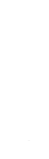
. From the above mentioned properties, it results that if one knows the arc

of trajectory between two consecutive apsides, then one may set up geometrically the

whole trajectory (Fig.8.3). From (8.1.2) it results that



has a constant sign, so that the

particle is rotating always in the same direction around the point

O . A bounded orbit is

closed if, after a finite number of such rotations, the particle returns to a previous

Dynamics of the particle in a field of elastic forces

475

position; thus, the condition

22qχπ

∈



must be satisfied. Otherwise, the orbit

is open and covers the annulus

[

]

max

min

,rrr

∈

. We also notice that the apparent

potential

()Ur has a maximum at a point in the interior of the annulus, corresponding

() d ()/d 0Fr Ur r==. We mention that the equation () 0rϕ

can have more

than two roots (the case of the constant

h of energy, Fig.8.2). In this case, one obtains

two possible annular domains (contained between the circles of radii

r and

r or

and

r , respectively); the motion takes place in that domain in

Figure 8.3. Orbit of a particle acted upon by a central force.

which is the initial position given by

()rrt

. If

min

, then the particle passes

through the pole

O or stops at that point. Assuming that 0C

≠

(otherwise, the

trajectory is rectilinear), the term

/2mC r− allows to have

lim ( )

→

=−∞, the

“falling” towards

O being thus hindered. The condition of “falling” towards O is

given by the condition

Uh≥− , written in the form

222

() /2rU r mC hr−≥−. To

have

min

it is necessary that

lim ( )

rU r

→+

≥

⎡⎤

⎣⎦

hence that ()Ur tends to zero at least as

/Ar,

/2AmC> , or as /

Ar, 0A > ,

2n >

max

min

rr r

= , then the trajectory is a circle of radius

r , corresponding

() 0Fr =

and the constant of energy

max

hU=−

(Fig.8.2); the considerations made

at the previous subsection remain valid.

One may prove

MECHANICAL SYSTEMS, CLASSICAL MODELS

476

Theorem 8.1.1 (J. Bertrand). The only closed orbits corresponding to central forces

are those for which

2s =−

, in any initial conditions, or

1s =

0k >

, in

certain initial conditions, assuming a potential of the form

() /

Ur k r

constk =

s ∈ 

1.1.3 Case of a force the modulus of which is in inverse proportion to the square of

the distance to a fixed point

Jacobi has considered the case in which the central force is of the form

()/Frγθ= , hence it is in inverse proportion to the square of the distance to the pole

O . Binet’s equation (8.1.4) takes the form

(

)

()

d1 1

γθ

+=− ;

(8.1.12)

by integration, one obtains

cos sin ( )CC

θθγθ=++,

(8.1.12')

where

()γθ is a particular integral, which may always be calculated by quadratures.

The integration constants are easily obtained by initial conditions of Cauchy type.

Analogously, we may consider central forces of the form

/kr, constk = , which

lead to the equation

(

)

(

)

d1 1

+=,

(8.1.13)

wherefrom it results the general integral

cos sinCC

βθ βθ=+,

1/kmCβ =+ .

(8.1.13')

1.2 Other problems

We consider now two other problems, i.e.: the problem of two particles, which leads

to the classical case of action of central forces and the problem of motion of a particle

subjected to the action of a central force in a resistent medium. We study the

phenomena of capture and diffraction too.

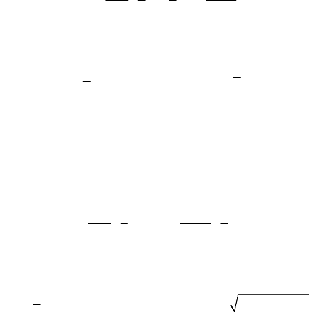
1.2.1 The problem of two particles. Capture. Diffraction

Let be two bodies which may be modelled by two particles

P and

P of position

vectors

r and

r and of masses

m and

m , respectively (Fig.8.4). We suppose that

this system of particles is acted upon only by the internal forces

21 12 12 21

vers versFF=− = =−FF r r,

12 2 1 21

−=−rrr r, where 0F > in case

Dynamics of the particle in a field of elastic forces

477

of repulsive forces and

in case of forces of attraction. From the equations of

motion

11 21

m =−



22 21



, amplifying by

m and

m , respectively, and

subtracting, one obtains

12 21

m =



21 12



111

mm m

=+,

(8.1.14)

where

m is the reduced mass. These equations describe the motion of the particle

with respect to the particle

P (as if the latter one would be fixed), as well as the motion

of the particle

P with respect to the particle

P ; in such conditions, the force

F and

the force

F are central forces, respectively, and one may use the results previously

obtained.

Figure 8.4. Problem of the two particles.

These considerations allow to study also the case in which

max

r is not finite, the

orbit being unbounded. We must have

lim ( ) lim ( )

hUr UrU

∞

→∞ →∞

−≤ = = . To fix the

ideas, we assume that

∞

; because the integral ()d

UFrr

∞

∫

must have a

sense, we suppose that

tends to zero for r →∞ at least as

1/r

ε+

0ε >

. The

condition of “escape” at infinity becomes

0h ≥

. Indeed, if we assume that the particle

is situated at the centre

, while the particle

tends to infinity, the interaction

ceases and one has

∞

= ; the particle

is endowed, in this case, only with kinetic

energy

, so that

0Th=≥

. The symmetry of the trajectory with respect to the line

of the pericentre remains valid (the same as in the case of bounded orbits); we notice

that the unbounded orbits have only one pericentre and pass only once through it.

If the particle

comes from infinity and enters in interaction with the particle

then may appear the phenomenon of capture (

remains finite or vanishes for

t →∞) or the phenomenon of diffraction (r →∞ for t →∞). We notice that

Cbv

h =

(8.1.15)

where

=−vv v is the relative velocity at the initial moment, while b is the

distance from

P to the support of the velocity. The formula (8.1.6''') where we take

MECHANICAL SYSTEMS, CLASSICAL MODELS

478

0t = gives the time in which the particle coming from infinity reaches a position at

finite distance in the form

()

ϕρ

−∞

=−

∫

;

(8.1.16)

we noticed that the radial velocity is directed towards the particle

. One has a real

motion only if

() 0rϕ > ; we observe that

()2/ 0hm vϕ

−

∞= = >

. Thus, if the

time

t increases, then the radius vector r decreases.

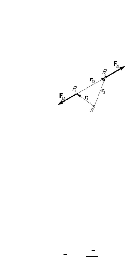
Figure 8.5. Capture: at a pole (a); on a circle (b).

For

t →∞ we may have 0r → , obtaining the phenomenon of capture; the

trajectory of the particle

P is thus a spiral which tends to the pole O (Fig.8.5,a). But if

there exists a radius

r for which () 0rϕ

, then we may write

() ( ) ()rrr r

ϕψ=− , () 0rψ

≠

. The integral (8.1.16) is divergent if 2ν ≥ , while

rr→ for t →∞; we obtain a phenomenon of capture too in which the trajectory of

the particle

P is also a spiral wrapped up a circle of radius rr

(Fig.8.5,b). The

phenomenon of capture may take place only in case of forces of attraction between the

two particles.

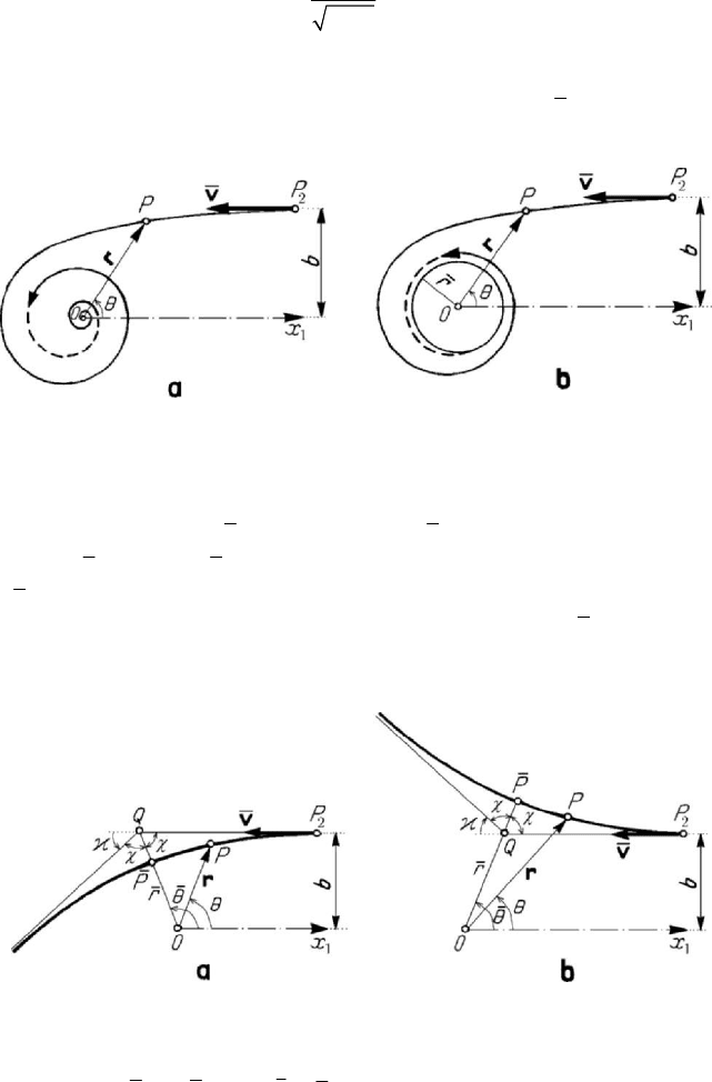
Figure 8.6. Diffraction: force of attraction (a); repulsive force (b).

2ν < , then the integral (8.1.16) is convergent so that there exists a finite moment

t for which rr= , () 0rϕ

(

min

is the minimal value of r corresponding

Dynamics of the particle in a field of elastic forces

479

to a constant of energy

h , Fig.8.2); the respective point P is a pericentre, while the

apsidal line

OP is a symmetry axis of the trajectory, which has the form in Fig.8.6,a, in

case of forces of attraction, or the form in Fig.8.6,b, in case of repulsive forces. One

obtains thus the phenomenon of diffraction. The apsidal angle is expressed in the form

χπθ=−, in case of a force of attraction, and by χθ

, in case of a repulsive force,

where the angle

θ is given by the formula (8.1.6'')

()

−∞

∫

1()0

mv b

⎛⎞

−

⎜⎟

⎝⎠

(8.1.17)

The angle



formed by the asymptotic direction of the trajectory with the support of

the velocity

v (in fact, the angle of the two asymptotes to the trajectory) is called

diffraction angle and is given by

(2)πθ=−∓



, where one takes the sign – or the

sign + as the diffraction is of attraction or is repulsive, respectively. If we denote by

“prime” the quantities which intervene after the interaction (for

t →∞), the relations

(8.1.15) show that

′

= , vv

′

; hence, the magnitude of the relative velocity is

conserved, the velocity vector changing only with the diffraction angle.

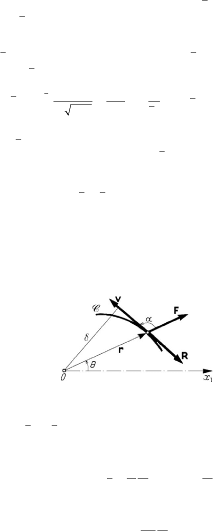
1.2.2 Motion of a particle acted upon by a central force in a resistent medium

This case of motion generalizes the case previously considered; obviously, it leads to

a plane trajectory

C too, the resistance R of the medium being tangent to the

trajectory and opposed to the motion (Fig.8.7). Hence, the equation of motion is of the

form

Figure 8.7. Particle acted upon by a central force in a resistent medium.

mF R

=−





, (,,, ;)FFrrtθθ=



, (,,, ;)RRrrtθθ=



;

(8.1.18)

in polar co-ordinates, we have

()

mr r F R

θ−=−





()

rt v

=−



(8.1.18')

Eliminating the resistance

R between these equations, it results

()

Fmrr r

θθ

⎡

⎤

=−−

⎢

⎥

⎣

⎦







MECHANICAL SYSTEMS, CLASSICAL MODELS

480

We return to the calculus in Subsec. 1.1.1 and assume that



; hence, we get

()

() ()

22 2

d1 1 d1 1

Fmv

rr rr

θθ

⎡⎤⎡⎤

=− + =− +

⎢⎥⎢⎥

⎣⎦⎣⎦



(8.1.19)

generalizing thus Binet’s formula (8.1.8).

In this case, the areal velocity is no more constant (we can no more write a first

integral of areas). Noting that

/2rΩθ=



, the second equation (8.1.18') leads to

(ln )

tmv

Ω

==−



(8.1.20)

We observe that

/2vΩδ= , where δ is the distance from the pole O to the support

of the velocity

(Fig.8.7); we may write

Ω

=−



(8.1.20')

too, so that the resistance of the medium is in direct proportion to the areal acceleration;

as well, we obtain the relation

(

)

4d 2

Ω

ΩΩ

δδ

=− =− .

(8.1.20'')

In particular, in case of a resistance of the form

Rkmv= , constk

, 0k > , we

obtain

d(ln ) d dkv t k sΩ =− =− , where s is the curvilinear co-ordinate along the

trajectory; it results

eΩΩ

−

(8.1.21)

so that the areal velocity decreases exponentially.

2. Motion of a particle subjected to the action of an elastic

force

In case of a conservative central force for which

() /2Ur kr=− or

() /2Ux kx=− , 0k > (one of the two cases considered in Bertrand’s theorem), one

obtains an elliptic oscillator (with two degrees of freedom) or a linear oscillator (with

only one degree of freedom), respectively; the force which derives from this potential is

an elastic force. We consider also the corresponding damped and sustained (including

self-sustained) oscillations. A particular attention is given to repulsive elastic forces

(

0k < ), as well as to a study of non-linear oscillations.

Dynamics of the particle in a field of elastic forces

481

2.1 Mechanical systems with two degrees of freedom

In what follows, we study the non-damped and damped elliptic oscillator, in case of

elastic forces of attraction as well as in case of repulsive elastic forces; the case of self-

sustained oscillations is also taken into consideration.

2.1.1 Elliptic oscillator

In case of central forces of the form

()versFr

Fr, we may assume for ()Fr a

development into a Maclaurin series

(0) (0)

( ) (0) ...

1! 2 !

Fr F r r

′

′′

=+ + +

(8.2.1)

We take

(0) 0F = , assuming that the pole O is a position of equilibrium. In case of

small motions (for which

1r  , the unit having the dimension of a length) we neglect

the powers of higher order. We denote

(0)Fk

′

− , 0k > ; the force is thus directed

towards the centre

O , considering that one as a stable position of equilibrium. A force

of the form

verskr k

−=−Frr

(8.2.2)

is called elastic force (in fact, in the following, by elastic force we mean an elastic force

of attraction).

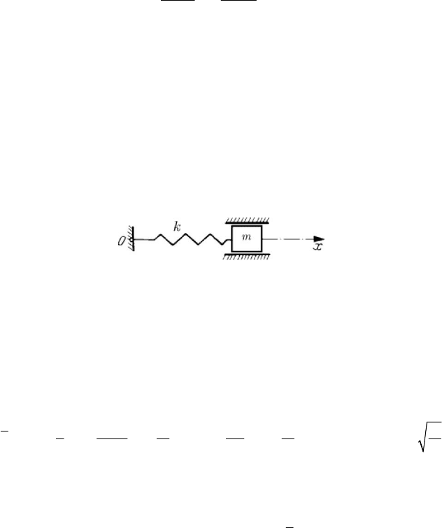
Figure 8.8. Model of an elastic force.

In the case in which the force

F has a fixed support (along the Ox -axis) we may

write

()Fx kx=− , modelling thus the force by an elastic spring of elastic constant

(coefficient of elasticity)

k , fixed at one end and acted upon by a force F due to a mass

m at the other end; the particle is modelled by a rigid body the motion of which is

guided (Fig.8.8). The denomination given to this force is thus justified.

The corresponding apparent potential is

()

222222

()

22 2

kmC m C m

Ur r r r

ωωθ

⎛⎞

=− − =− + =− +

⎜⎟

⎝⎠



ω =

(8.2.3)

where we have taken into consideration the constant of areas (8.1.2); the graphic of this

function is given in Fig.8.9, where the graphics of the two component terms are put into

evidence. In case of a constant of energy

h for which ()Ur h≥− we obtain a bounded