Teodorescu P.P. Mechanical Systems, Classical Models Volume I: Particle Mechanics

Подождите немного. Документ загружается.

MECHANICAL SYSTEMS, CLASSICAL MODELS

492

()

lim e cosh lim e 1 e

ttt

λωλω

−−−−

→∞ →∞

+=∞;

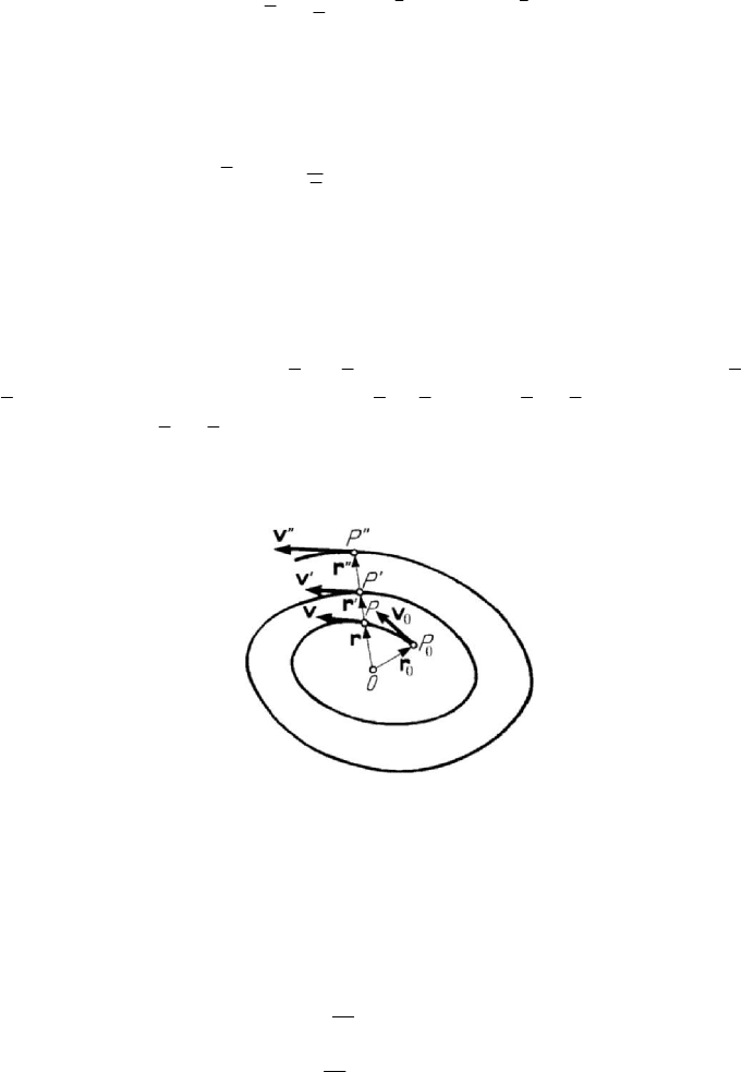
hence, the trajectory is similar to that in Fig.8.12 (the arc of hyperbola is deformed, the

radii being smaller), but it is travelled through with a smaller velocity. The asymptote to

which tends the trajectory is specified by the vector (Fig.8.14)

000

()λ

=+ +

rr v r.

(8.2.18

)

2.1.4 Self-sustained motions of a particle

Various types of motion considered in Subsecs 2.1.1 and 2.1.2 may be due to a given

perturbing force, the respective motion being a forced (sustained) motion. If the force

which maintains the motion is due to the motion itself, being of the form

′



rΦ ,

′

> , then the motion is called a self-sustained motion; in fact, the force Φ is of the

form

′′′

ΦΦ, where k

′

−



rΦ , 0k

′

> , is a damped force, while k

′′ ′′



rΦ ,

′′

, is a perturbing force, with

0kkk

′′′′

−>

(if

′

′′

, then the motion is

damped, while if

′′ ′

= , then the motion is non-damped). If the motion ceases, then

the corresponding force disappears. We observe that in a forced motion that force exists

independent of the motion and persists after its suppression.

Figure 8.15. Non-damped pseudoelliptic oscillator.

In case of an elastic force of attraction, the equation of motion is of the form

2λω

−

 

rrr0,

(8.2.19)

where we use the notations of the preceding subsection. With the initial conditions

(8.2.5'), we obtain

000

() e cos ( )sin

tt t

ωλω

⎡⎤

′

=+−

⎢⎥

′

⎣⎦

rr vr

(8.2.19')

000

() e cos ( )sin

tt t

ωωλω

⎡⎤

′

=−−

⎢⎥

′

⎣⎦

vv rv

(8.2.19'')

where we have introduced the pseudopulsation (8.2.15''), assuming that

ωλ> . The

trajectory is a spiral and the particle is rotating around the centre

O in the same

Dynamics of the particle in a field of elastic forces

493

direction till infinity (Fig.8.15). After a pseudoperiod

2/T πω

′

, the particle returns

on the same half-straight line with a velocity which has always the same direction for

that line; the radii and the velocities are increasing in geometric progression of ratio

tλ

for the same half-straight line, the number

2/Tδλ πλω

′

= being a logarithmic

increment. The corresponding mechanical system may be called non-damped

pseudoelliptic oscillator; the respective motion of the particle is a pseudoperiodic non-

damped motion.

ωλ= , we may write

[

]

000

() e ( )

λ=+−rrvr,

[

]

000

() e ( )

λλ=+−vvvr,

(8.2.20)

while if

ωλ

we get

000

() e cosh ( )sinh

tt t

ωλω

⎡⎤

′

′′′

=+−

⎢⎥

′′

⎣⎦

rr vr

(8.2.21)

000

() e cosh ( )sinh

tt t

ωωλω

⎡⎤

′

′′′

=−−

⎢⎥

′′

⎣⎦

vv rv

(8.2.21')

where we used the notation (8.2.17). In both cases, one obtains an aperiodic non-

damped motion (Fig.8.14), the asymptote to which tends the trajectory being specified

by the vector

=−

(8.2.20')

in the first case, and by the vector

000

()λ

=+ −

′′

rr v r,

(8.2.21'')

in the second case, respectively.

In case of a repulsive elastic force, it results the equation of motion

2λω

−

−=

 

rrr0

(8.2.22)

where we used the same notations as above. We obtain

000

() e cosh ( )sinh

tt t

ωλω

⎡⎤

=+−

⎢⎥

⎣⎦

rr vr

(8.2.22')

000

() e cosh ( )sinh

tt t

ωωλ ω

⎡⎤

=++

⎢⎥

⎣⎦

vv rv

(8.2.22'')

where we have put the initial conditions (8.2.5') and have introduced the notation

(8.2.18'''). The motion of the particle is an aperiodic non-damped motion too (Fig.8.14);

the trajectory tends to an asymptote specified by the vector

MECHANICAL SYSTEMS, CLASSICAL MODELS

494

000

()λ

=+ −rr v r

(8.2.22''')

2.2 Mechanical systems with a single degree of freedom

Projecting the motion of an elliptic oscillator on an axis in the plane of the

corresponding trajectory, we obtain a linear oscillator, the most simple mechanical

system with a single degree of freedom. We pass then to the case of a damped oscillator

and to that of a sustained one. The phenomena of interference and of beats will be taken

into consideration too, as well as the superposition of effects, which leads to small

oscillations of a particle around a stable position of equilibrium.

2.2.1 Linear oscillator

We consider a particle acted upon by an elastic force with a fixed support, chosen as

Ox -axis (of the form ()Fx kx

− , 0k > ), modelled as in Fig.8.8. With the notations

in Subsec. 2.1.1, the equation of motion has the form

0xxω

= ;

(8.2.23)

with the initial conditions

(0)xx

(0)vv

(8.2.23')

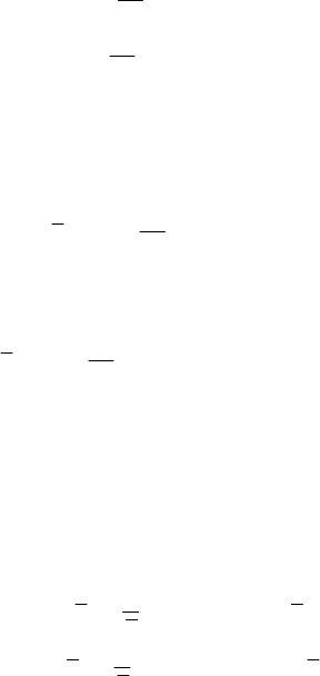
Figure 8.16. Linear oscillator: trajectory (a); diagram ()xt vs ()tb .

we may write

cos sin cos( )

xx t ta tωωωϕ

=+=−,

(8.2.24)

cos sin sin( )vv t x t a tωω ω ω ωϕ=− =−−,

(8.2.24')

where

=+,

arctan

(8.2.24'')

Dynamics of the particle in a field of elastic forces

495

are the amplitude of the oscillation (maximal elongation, the elongation

x being the

distance from the centre of oscillation

O to the position of the particle at a given

moment) and the phase shift (the argument

tωϕ

−

represents the phase at the moment

t , the phase shift being calculated with respect to the phase tω ), respectively. The

trajectory is the segment of line

AA , which is travelled through back and forth in the

period of time (8.2.6), beginning with the initial position

P (Fig.8.16,a). We have thus

to do with oscillations around the oscillation centre

O , which is a stable position of

equilibrium. Because the period

T (and the frequency 1/Tν

) is independent on

the amplitude, it results that the free linear oscillations with a single degree of freedom

are isochronic; on the other hand, the interval of time

/4T in which the segment of

line

AO is travelled through does not depend on the initial position A (does not

depend on

a ), the velocity at that point vanishing, so that the motion is tautochronous

too.

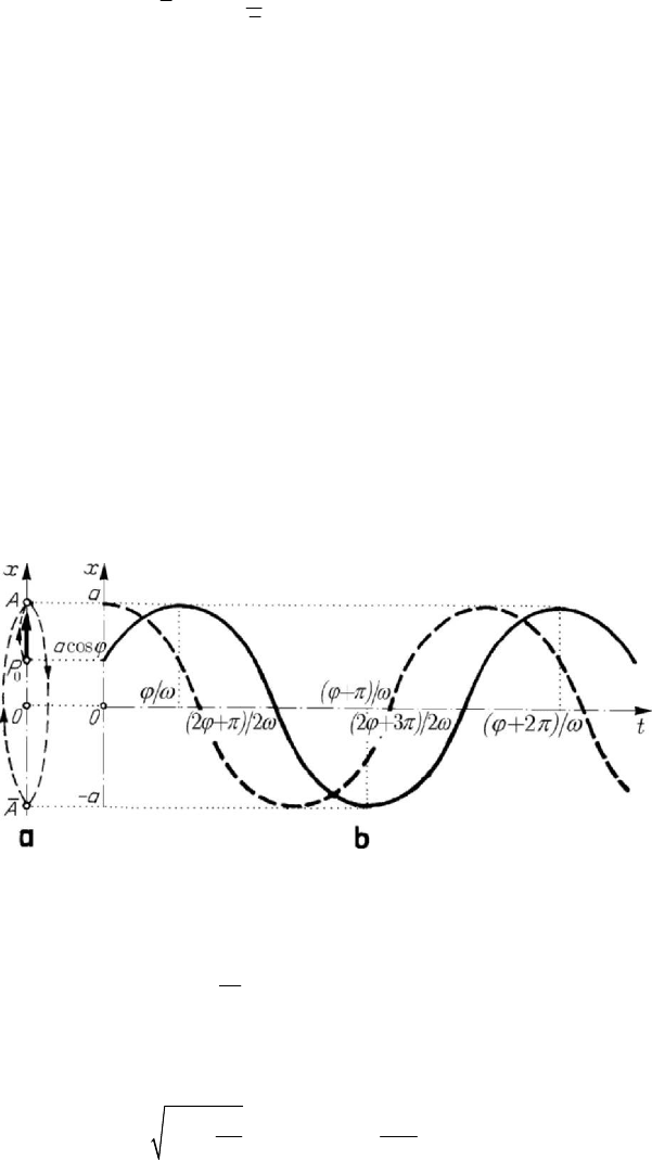
Figure 8.17. Linear oscillator as projection of a circular oscillator.

The mechanical system formed by a particle which describes a segment of a line,

subjected to the action of an elastic force is called linear oscillator; that one may be

also considered as a limit case of an elliptic oscillator, namely that in which one of the

semiaxes of the ellipse tends to zero. We notice that a linear oscillator may be obtained

too by projecting the motion of a circular oscillator (hence, of a particle

′

with a

velocity v of constant modulus

aω

, which is in uniform motion on a circle) on a

diameter

of it (Fig.8.17); if the position of the diameter

is specified by the

angle

ϕ with respect to the

Ox -axis and if the angle tθω

, where ω is the angular

velocity, gives the position of the radius

′

, then we obtain the equation (8.2.24) of

the linear oscillator. Any mechanical system with only one degree of freedom subjected

to small oscillations around a stable position of equilibrium, e.g., the simple pendulum

subjected to small oscillations, may be modelled by a linear oscillator.

Multiplying the equation (8.2.23) by

mx , we obtain

(

)

d2 2

mxx kxx x x

+= +

   ,

so that, taking into account (8.2.6'), (8.2.24) and (8.2.24'),

MECHANICAL SYSTEMS, CLASSICAL MODELS

496

2222

ETUTV a ma

πν=−=+= = ;

(8.2.23'')

it results that, during the non-damped free linear oscillations with a single degree of

freedom, a process of conservation of the mechanical energy takes place.

In general, a motion with a single degree of freedom of a mechanical system

represents a harmonic vibration (harmonic oscillation, the term of oscillation being

usually used if the particle returns always on the same trajectory) if it is of the form

(8.2.24); we mention also that the term of oscillation may be used also for non-

mechanical oscillations, but the term of vibration is used only for mechanical ones. The

diagram of the considered motion is represented in Fig.8.16,b by a unbroken line

(comparing with the dash line which corresponds to the vibration

cosxa tω=

, the

influence of the phase shift being thus put into evidence).

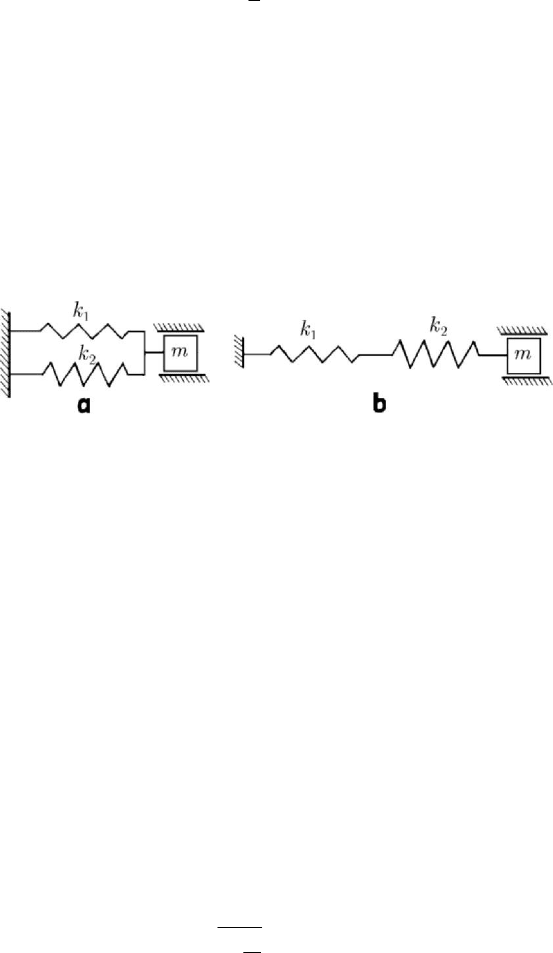
Figure 8.18. Model of a system of linear oscillators: parallel linkage (a); linkage in series (b).

Some vibrating mechanical systems may be physically modelled by a system formed

of several elastic elements, of negligible masses, linked between them; such a system

can be replaced, in general, by a single equivalent elastic element. In case of two

springs of elastic constants

k and

k , respectively, linked in parallel (Fig.8.18,a), the

condition that the total elastic force for a displacement

x be equal to the sum of the

forces corresponding to each spring (

kx k x k x

+ ) is put, wherefrom

kk k=+.

In case of

n springs linked in parallel, we may write ( /kn is an arithmetic mean)

∑

(8.2.25)

If the two springs are linked in series (Fig.8.18,b), then the condition that the total

elongation

x of the spring be equal to the sum of the elongations

x and

x , of the

component springs, respectively, is put (

xx x

+ ), the force in the spring being the

same along it (

11 22

kx k x k x=+

); it results

1/ 1/ 1/kk k

+ . In case of n springs

linked in series, we obtain (

is a harmonic mean)

∑

(8.2.25')

Dynamics of the particle in a field of elastic forces

497

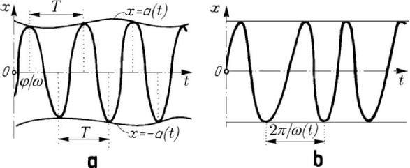
2.2.2 Modulated vibrations

In case of the motion of a mechanical system with a single degree of freedom, of the

form

() ()cos( )xt at tωϕ

− ,

(8.2.26)

we say that we have to do with a vibration modulated in amplitude; in general, we

assume that

()at varies little in the quasi-period 2/T πω

. The diagram of motion

(the trajectory of which is also a segment of a line, as in the preceding case) has the

aspect of a cosinusoid which is contained between the curves

()xat

± (Fig.8.19,a).

We notice that the function (8.2.26) and its derivative

() ()cos( )xt at tωϕ

−

()sin( )at tωωϕ−− have values equal to those of the functions () ()xt at=± and of

the respective derivatives

() ()xt at

± at the points of abscissae /t ϕω= ,

/tTϕω=+,… and //2tTϕω=+, /3/2tTϕω

+ ,…, respectively; hence,

the diagram of motion is tangent to the curves

()xat

± . The intervals between two

successive points of tangency are equal to

T , as well as the intervals between two

points in which the

Ot -axis is pierced in the same direction. The respective motion is a

quasi-periodic motion. Eventually, even the function

()xat

may be periodic.

Figure 8.19. Modulated vibration: in amplitude (a); in frequency (b).

If the motion is definite in the form

[

]

() cos ()xt a ttωϕ

− ,

(8.2.26')

then we say that it is a vibration modulated in frequency (or modulated in phase); in

general, one assumes that

()tω varies little in a pseudoperiod 2/()Ttπω

. We may

have, for instance,

() sinttωωεω=+ ,

/1εω . The diagram of motion has the

aspect in Fig.8.19,b.

2.2.3 Representations of harmonic vibrations

We have seen in Subsec. 2.2.1 that a harmonic vibration may be obtained by

projecting a circular oscillator on one of its diameters; this observation has led Fresnel

MECHANICAL SYSTEMS, CLASSICAL MODELS

498

to elaborate a vector method of representation of harmonic vibrations; this method is

particularly useful for the composition of these vibrations.

Thus, the harmonic vibration (8.2.24) may be represented by the vector





modulus

OQ a=





, the direction of which is given by the angle

tθω ϕ=−

, taken

counterclockwise from the

-axis, which represents the phase of motion; this vector

of constant modulus has a uniform rotation around the pole

, in positive or negative

sense, as the angular velocity

0ω ≷

. If the point Q is projected at

on the

axis, then

OP x=

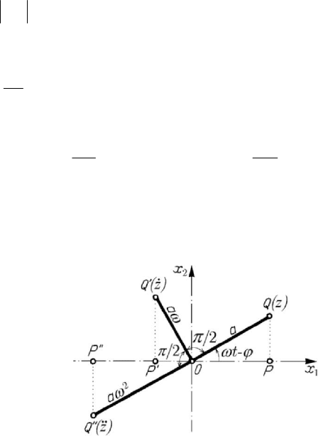
(Fig.8.20). Observing that

sin( )xa tωωϕ=− − ,

cos( )xa tωωϕ=− − ,

it results the velocity

OP x

′

 and the acceleration OP x

′′

 , which correspond to a

vector

′





of modulus aω , the direction of which is obtained by rotating of /2π the

vector





counterclockwise or clockwise as 0ω ≷ or to a vector OQ

′′





of modulus

aω

, opposite to the vector OQ





, respectively.

Figure 8.20. Vector representation of harmonic vibrations.

If we assume that the above vector representation is made in the complex variables

plane, then to the point

Q , hence to the vector OQ





, there corresponds the variable

izx x=+

; we may thus write (Fig.8.20)

[]

i( )

cos( ) i sin( ) e

za t t a

ωϕ

ωϕ ωϕ

−

=−+−=

(8.2.27)

where

−

is the complex amplitude of the oscillation. Differentiating successively,

we obtain

[]

i( ) i( /2)

sin( ) i cos( ) ie e

za t t a a

ωϕ ωϕπ

ωωϕ ωϕω ω

−−+

=− −+ −= =



(8.2.27')

[]

22i()

cos( ) i sin( ) e

za t t a

ωϕ

ωωϕ ωϕ ω

−

=− − + − =−



2i( )

ωϕπ

−

(8.2.27'')

Dynamics of the particle in a field of elastic forces

499

finding again the points

′

and Q

′

, respectively.

2.2.4 Composition of harmonic vibrations of the same direction. Interference.

Beats. Harmonic analysis

We consider first of all two harmonic vibrations

11 1

cos( )xa tωϕ=−,

22 2

cos( )xa tωϕ

− ,

which have the same direction and the same pulsation; their amplitudes and their phase

shifts may be different. By the composition of these vibrations (in case of acoustic or

light waves, the phenomenon is called interference too) we obtain also a harmonic

vibration

cos( )xx x a tωϕ=+= −, where

12 12 21

2cos( )aaa aa ϕϕ=++ −,

1122

sin sin

arctan

cos cos

ϕϕ

(8.2.28)

The term

12 2 1

2cos( )aa ϕϕ− is called the term of interference and leads to an effect of

interference stripes. If

2nϕϕ π

−

= , n

∈

 , then we obtain

aa a

, while if

(2 1)nϕϕ π−= + , n ∈  , then we have

aaa

− ; in the first case the

interference is constructive, while in the second one it is destructive. Finally, if

aa= , then the destructive interference leads to extinction (zones in which the sound

disappears, in case of acoustic waves, or zones of darkness, in case of light waves). If

/2nϕϕ π−= ,n ∈  , then

aaa=+,

(

)

arctan /aaϕ

. By composition

of a certain number of harmonic vibrations one may effect an analogous computation.

If the two harmonic vibrations have not the same pulsation, being of the form

11 1 1

cos( )xa tωϕ=−,

22 2 2

cos( )xa tωϕ

− ,

then their composition (by extension, the phenomenon bears the denomination of

interference too) leads to an expression of the same form, modulated both in amplitude

()()

[]

12 12 12 12

() 2 cosat a a aa tωω ϕϕ=++ − −−

(8.2.29)

and in phase

(

)

(

)

()()

12 12

1122

12 12

1122

sin sin

( ) arctan

cos cos

atat

ωω ωω

ϕϕ

ωω ωω

ϕϕ

−

−−+ +

−−

−+ +

(8.2.29')

where

(

)

/2ωωω

+ . The motion thus obtained is no more harmonic, its form

depending on the amplitudes, on the frequencies ratio, and on the phase shifts; it is a

periodic motion only if the periods of the two component motions have a common

MECHANICAL SYSTEMS, CLASSICAL MODELS

500

multiple, hence only if

11 22

2/ 2/nnπω πω

,nn

∈

 or

/ nωω= ,

n ∈ 

(Figs.8.21, 8.22). The amplitude

()at has a variation between

min 1 2

aaa=− and

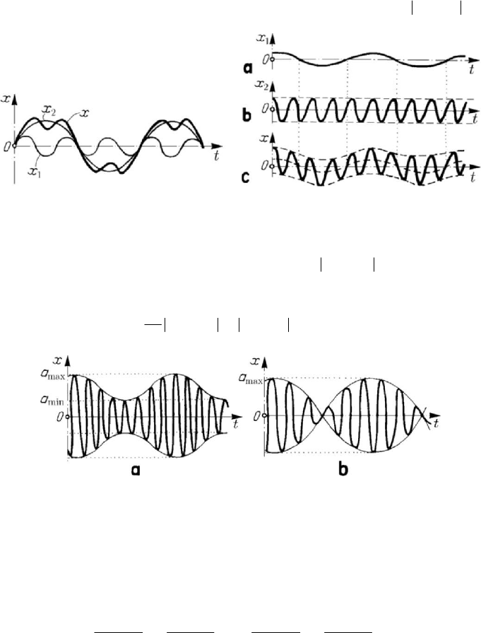
Figure 8.21-8.22. Composition of two harmonic vibrations for which

/ nωω= , n ∈  .

max

aaa=+, having maximal values (called beats in case of acoustic waves) at

intervals of time given by the period

T πω ω

− (Fig.8.23,a); the

corresponding frequency is

12 12

νωωνν

=−=−

(8.2.29'')

Figure 8.23. Beats: general case (a); simple beats (b).

hence it is equal to the absolute value of the difference of the frequencies of the

component motions. One may thus syntonize two musical instruments (the period of the

beats tends to infinity if the frequencies of the two instruments tend to be equal). The

phenomenon is as much perceptible as the two amplitudes are closer. If

aaa==,

then the formulae (8.2.29), (8.2.29') lead to

(

)

(

)

12 12 12 12

2cos cos

22 22

xa t t

ωω ϕϕ ωω ϕϕ−− ++

=− −

(8.2.30)

hence to a product of two harmonic functions. In this case,

max

2aa= , while

min

0a = (one obtains the node of the beat), the diagram of the motion being given in

Fig.8.23,b; the beats are simple beats.

Dynamics of the particle in a field of elastic forces

501

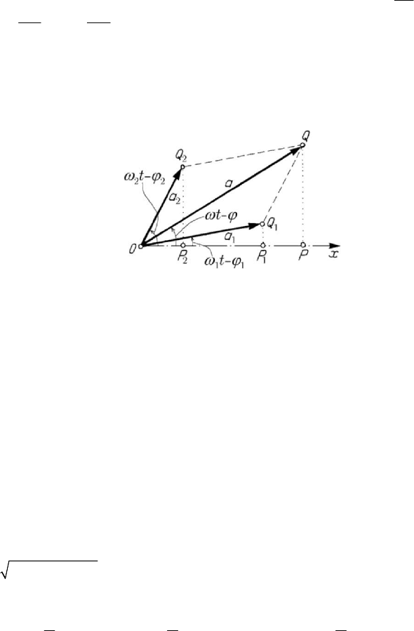
Using Fresnel’s method of representation, we can compose the vectors





and





, obtaining the vector OQ





, to which corresponds the motion

xOPx x

xOP= ,

xOP= (Fig.8.24). Analogously, one may compose an arbitrary number

of harmonic vibrations

cos( )

ii i i

xa tωϕ

− , 1,2,...,in

. The resultant motion is

not – in general – harmonic, neither periodic; the motion is periodic if and only if the

ratio between any two pulsations is a rational number (

ij ij

nωω=

n ∈  ,

, 1,2,...,ij n∀= ).

Figure 8.24. Fresnel’s representation method.

The inverse problem, which consists in the determination of the harmonic

components of a given periodic motion

()()xt T xt

= forms the object of harmonic

analysis; this problem is of particular importance in physics, in engineering technology

etc. Assuming that Lejeune-Dirichlet’s sufficient conditions (the function

()xt is

piecewise continuous, having a finite number of points of discontinuity of the first kind

and a finite number of maxima and minima on the time interval

) are fulfilled, we

may decompose the motion in the form

112 2

() cos( ) cos(2 ) ...xt a a t a tωϕ ωϕ=+ − + − +

... cos( ) ...

antωϕ+−+

(8.2.31)

where

2/Tωπ

. We obtain thus a finite Fourier representation (an example of

decomposition of a periodic motion in a sum of two harmonic vibrations is given in

Fig.8.21) or a development into a Fourier series; the amplitudes

() ()

′′′

=+ and the phase shifts

(

)

arctan /

nnn

aaϕ

′

′′

are expressed by

means of the Fourier coefficients

()d

axtt

∫

()cos d

axtntt

′

∫

()sin d

axtntt

′′

∫

(8.2.31')

where the integration is effected along a period, beginning from an arbitrarily chosen

point; the coefficient

a represents the mean value of the displacement ()xt . The

oscillation

cos( )atωϕ− is of minimal frequency

min

/2νωπ

(of maximal period