Vidakovic B. Statistics for Bioengineering Sciences: With Matlab and WinBugs Support

Подождите немного. Документ загружается.

10.3 Testing the Equality of Normal Means When Samples Are Paired 369

sqrt(co(1,1) + co(2,2) - 2

co(1,2))

%ans =3.6904

We remark that the assumption of equality of population variances is not

necessary since we operate with the differences, and the population variance

of the differences,

=σ

+σ

−2σ

, is unknown.

We are interested in testing the means, H

: µ

=µ

, versus one of the three

alternatives H

: µ

>,6=,< µ

. Under H

the test statistic t has a t distribu-

tion with n

−1 degrees of freedom. Thus, the test coincides with the one-sample

t-test, where the sample consists of all differences and where H

is the hypoth-

esis that the mean in the population of differences is equal to 0. The popular

name for this test is the paired t-test, which can be summarized as follows:

Alternative α-level rejection region p-value

: µ

>µ

n−1,1−α

,∞) 1-tcdf(t, n-1)

: µ

6=µ

(−∞, t

n−1,α/2

] ∪[t

n−1,1−α/2

,∞) 2

tcdf(-abs(t), n-1)

: µ

<µ

(−∞, t

n−1,α

] tcdf(t, n-1)

One can generalize this test to testing H

: µ

−µ

= d

versus the appro-

priate one- or two-sided alternative. The only modiﬁcation needed is in the

t-statistic (10.7), which now takes the form

d −d

which under H

has a t distribution with n −1 degrees of freedom.

δ = µ

−µ

is the difference between the population means, then the

−α)100% conﬁdence interval for δ is

d −t

n−1,1−α/2

, d +t

n−1,1−α/2

Since matching (blocking) the observations eliminates the variability be-

tween the subjects entering the inference, the paired t-test is preferred to a

two-sample t-test whenever such a design is possible. For example, the case-

control study design selects one observation or experimental unit as the “case”

variable and obtains as “matched controls” one or more additional observa-

tions or experimental units that are similar to the case, except for the vari-

able(s) under study. When the treatments are assigned after subjects have

been paired, this assignment should be random to avoid any potential system-

atic inﬂuences.

370 10 Two Samples

Example 10.5. Psoriasis. Woo and McKenna (2003) investigated the effect

of broadband ultraviolet B (UVB) therapy and topical calcipotriol cream used

together on areas of psoriasis. One of the outcome variables is the Psoriasis

Area and Severity Index (PASI), where a lower score is better. The following

table gives PASI scores for 20 subjects measured at baseline and after 8 treat-

ments. Do these data provide sufﬁcient evidence, at a 0.05 level of signiﬁcance,

to indicate that the combination therapy reduces PASI scores?

Subject Baseline After 8 treatments Subject Baseline After 8 treatments

1 5.9 5.2 11 11.1 11.1

2 7.6 12.2 12 15.6 8.4

3 12.8 4.6 13 9.6 5.8

4 16.5 4.0 14 15.2 5.0

5 6.1 0.4 15 21.0 6.4

6 14.4 3.8 16 5.9 0.0

7 6.6 1.2 17 10.0 2.7

8 5.4 3.1 18 12.2 5.1

9 9.6 3.5 19 20.2 4.8

10 11.6 4.9 20 6.2 4.2

The data set is available as pasi.dat|xls|mat.

We will import the data into MATLAB and test the hypothesis that the

PASI signiﬁcantly decreased after treatment at a signiﬁcance of

α = 0.05. We

will also ﬁnd a 95% conﬁdence interval for the difference between the popula-

tion means

δ =µ

−µ

baseline = [5.9 7.6 12.8 16.5 6.1 14.4 6.6 5.4 ...

9.6 11.6 11.1 15.6 9.6 15.2 21 5.9 10 12.2 20.2 6.2];

after = [5.2 12.2 4.6 4 0.4 3.8 1.2 3.1 3.5 4.9 ...

11.1 8.4 5.8 5 6.4 0 2.7 5.1 4.8 4.2];

d = baseline - after;

n = length(d);

dbar = mean(d) %dbar = 6.3550

sdd= sqrt(var(d)) %sdd = 4.9309

tstat = dbar/(sdd/sqrt(n)) %tstat = 5.7637

% Test using RR

critpt = tinv(0.95, n-1) %critpt = 1.7291

% Rejection region (1.7291, infinity). Reject H

0 since

% tstat=5.7637 falls in the rejection region.

% Test using the p-value

value = 1-tcdf(tstat, n-1) %p

value = 7.4398e-006

% Reject H

0 at the level alpha=0.05

% since the p

value = 0.00000744 < 0.05.

alpha = 0.05

LB = dbar - tinv(1-alpha/2, n-1)

(sdd/sqrt(n))

% LB = 4.0472

UB = dbar + tinv(1-alpha/2, n-1)

(sdd/sqrt(n))

10.3 Testing the Equality of Normal Means When Samples Are Paired 371

% UB = 8.6628

% 95% CI is [4.0472, 8.6628]

Alternatively, if one uses d1=after-baseline, then care must be taken about

the “direction” of H

and p-value calculations. The rejection region will be

(

−∞,−1.7291) and the 95% conﬁdence interval [−8.6628,−4.0472].

A Bayesian solution is given next.

model{

for(i in 1:n){

d[i] <- baseline[i] - after[i]

d[i] ~ dnorm(mu, prec)

}

mu ~ dnorm(0, 0.00001)

pH1 <- step(mu-0)

prec ~ dgamma(0.001, 0.001)

sigma2 <- 1/prec;

sigma <- 1/sqrt(prec)

}

DATA

list(n=20,

baseline = c(5.9, 7.6, 12.8, 16.5, 6.1, 14.4, 6.6,

5.4, 9.6, 11.6 ,11.1, 15.6, 9.6, 15.2, 21, 5.9,

10, 12.2, 20.2, 6.2),

after = c(5.2, 12.2, 4.6, 4, 0.4 , 3.8, 1.2, 3.1, 3.5,

4.9, 11.1, 8.4, 5.8, 5, 6.4, 0, 2.7, 5.1, 4.8, 4.2))

INITS

list(mu=0, prec=1)

mean sd MC error val2.5pc median val97.5pc start sample

pH1 1.0 0.0 3.162E-13 1.0 1.0 1.0 1001 100000

mu 6.352 1.169 0.003657 4.043 6.351 8.666 1001 100000

prec 0.04108 0.01339 4.498E-5 0.01927 0.03959 0.07149 1001 100000

sigma 5.142 0.8912 0.003126 3.74 5.026 7.203 1001 100000

sigma2 27.23 10.0 0.03528 13.99 25.26 51.88 1001 100000

Let us compare the classical and Bayesian solutions. The estimator for the

difference between population means is 6.3550 in the classical case and 6.352

in the Bayesian case. The standard deviations of the difference are close as

well: the classical is 4.9309/

20 =1.1026 and the Bayesian is 1.169.

The 95% conﬁdence interval for the difference is [4.0472,8.6628], while the

95% credible set is [4.043,8.666].

The posterior probability of H

is approx. 1, while the classical p-value

(support for H

) is 0.000007439.

This closeness of results is expected given that the priors

∼

dnorm(0,0.00001)

and prec∼dgamma(0.001,0.001) are noninformative.

372 10 Two Samples

Next, we provide an example in which the measurements are taken on dif-

ferent subjects, but the subjects are matched with respect to some characteris-

tics that may inﬂuence the response. Because of this matching, the sample is

considered paired. This is often done when the application of both treatments

to a single subject is either impossible or leads to biased responses.

Example 10.6. IQ-Test Pairing. In a study concerning memorizing verbal

sentences, children were ﬁrst given an IQ test. The two lowest-scoring children

were randomly assigned, one to a “noun-ﬁrst” task, the other to a “noun-last”

task. The two next-lowest IQ children were similarly assigned, one to a “noun-

ﬁrst” task, the other to a “noun-last” task, and so on until all children were

assigned. The data (scores on a word-recall task) are shown here, listed in

order from lowest to highest IQ score:

Noun-ﬁrst 12 21 12 16 20 39 26 29 30 35 38 34

Noun-last

10 12 23 14 16 8 16 22 32 13 32 35

If µ

and µ

are population means corresponding to “noun-ﬁrst” and “noun-

last” tasks, we will test the hypothesis H

: µ

−µ

= 0 against the two-sided

alternative. The signiﬁcance level is set to

α =5%.

Note that the two samples are not independent since the pairing is based

on an ordered joint attribute, children’s IQ scores. Thus, even though the sub-

jects in the two groups are different, the paired t-test is appropriate.

% Noun First Example

disp(’Noun First Example’)

nounfirst = [12 21 12 16 20 39 26 29 30 35 38 34];

nounlast = [10 12 23 14 16 8 16 22 32 13 32 35];

d=nounfirst - nounlast;

dbar = mean(d)

%dbar = 6.5833

sd = std(d)

%sd = 11.0409

n = length(d)

%n = 12

t = dbar/(sd/sqrt(n))

%t = 2.0655

pval = 2

(1-tcdf(t, n-1))

%pval = 0.0633

The null hypothesis is not rejected against the two-sided alternative H

6=µ

at the 5% level. However, for the one-sided alternative, in this case H

>µ

, the p-value would be less than 5% and the null would be rejected. The

testing is equivalent to a one-sample t-test against the alternative

−µ

>0.

pval = 1-tcdf(t, n-1)

%pval = 0.0316

10.4 Two Variances 373

10.3.1 Sample Size in Paired t-Test

If in the paired t-test context the variance of the differences, σ

, were known,

then

d −d

∗

would have a standard normal distribution. Thus, to achieve a power of 1

−β

by an α-level test against the alternative H

: µ

−µ

= d

∗

, the one-sided test

would require

≥

1−α

1−β

)

∗

)

(10.8)

observations. For the two sided alternative, the standard normal quantile z

1−α

should be replaced by z

1−α/2

Example 10.7. Suppose that the study is to be designed for assessing the effect

of a blood-pressure-lowering drug in middle-aged men. Each subject will have

his systolic blood pressure (SBP) taken at the onset of the trial and after a

14-day regimen with the drug. In previous studies of related drugs, the vari-

ance of difference between the two measurements was found to be 300 (mm

Hg)

. The new drug would be of interest if it reduced the SBP by 5 mm Hg or

more.

What sample size is needed so that a 5% level test detects a difference of

5 mm Hg at least 90% of time?

Direct application of (10.8) with

= 300, d

∗

= 5, α = 0.05, and β = 0.1

gives a sample size of 103 subjects.

n = (300

(norminv(0.95) + norminv(0.9))^2 )/(5^2)

% 102.7662

10.4 Two Variances

We have already seen the test for equality of variances from two normal pop-

ulations when we discussed testing the equality of two independent normal

means.

We will not repeat the summary table (p. 359) but will talk about how to

ﬁnd a conﬁdence interval for the ratio of population variances, conduct power

analyses, and provide some Bayesian considerations.

Let s

and s

be sample variances based on samples X

, X

,... , X

1,n

and

, X

,... , X

2,n

from normal populations N (µ,σ

) and N (µ

,σ

), respec-

374 10 Two Samples

tively. The fact that the sampling distribution of

is F with df

= n

−1

and df

= n

−1 degrees of freedom was used in testing the equality of vari-

ances. The same statistic and its sampling distribution lead to a (1

−α)100%

conﬁdence interval for

/σ

, as

−1,n

−1,1−α/2

−1,n

−1,α/2

This follows from

−1,n

−1,α/2

≤

≤F

−1,n

−1,1−α/2

1 −α (10.9)

and the property of F quantiles,

m,n,α

n,m,1−α

Power Analysis for the Test of Two Variances

∗

. If F = s

is ob-

served, and n

and n

are sample sizes, Desu and Raghavarao (1990) provide

an approximation of the power of the test for the variance ratio,

−β ≈Φ

−1

2(n

−1)(n

−2)

−2

|log(F)|−z

1−α

, (10.10)

where z

1−α

is the 1 −α-quantile of the standard normal distribution. If the

alternative is two-sided, the quantile z

1−α/2

is used instead of z

1−α

The sample size necessary to achieve a power of 1

−β if the effect eff =

/σ

6=1 is to be detected by a test of level α is

1−α

1−β

log(eff)

+2. (10.11)

This size is for each sample, so the total number of observations is 2n. If un-

equal sample sizes are desired, the reader is referred to Zar (1996) and Desu

and Raghavarao (1990).

Example 10.8. In the context of Example 10.1, we approximate the power of

the two-sided, 5% level test of equality of variances against the speciﬁc alter-

native H

: σ

/σ

= 1.8. Recall that the group sample sizes were n

= 12 and

=15. According to (10.10),

10.4 Two Variances 375

n1 = 12; n2=15; alpha = 0.05; F = 1.8;

normcdf( sqrt(2

(n1-1)

(n2 -2)/(n1 + n2 -2 )) ...

abs(log(F)) - norminv(1-alpha/2) )

% 0.5112

and the power is about 51%.

Next we ﬁnd the retrospective power of the test in Example 10.2.

n1 = 12; n2=15; alpha = 0.05;

s12 = 0.004^2; s22 = 0.006^2;

F=s12^2/s22^2; %0.1975

normcdf( sqrt(2

(n1-1)

(n2 -2)/(n1 + n2 -2 )) ...

abs(log(F)) - norminv(1-alpha/2) )

% 0.9998

The retrospective power of the test is quite high, 99.98%.

If the lead exposure trial from Example 10.1 is to be repeated, we will

ﬁnd the sample size that would guarantee that an effect of size 1.5 would be

detected with a power of 90% in a two-sided 5% level test. Here the effect is

deﬁned as the ratio of population variances that is different than 1 and of

interest to detect.

alpha = 0.05; beta = 0.1; eff = 1.5;

n = ( (norminv(1-alpha/2) + norminv(1-beta))/log(eff))^2 + 2

% n=66 (65.9130)

Therefore, each group will need 66 children.

A Noninformative Bayesian Solution. If the priors on the parameters

are noninformative

π(µ

) = π (µ

) = 1,π(σ

) = 1/σ

, and π(σ

) = 1/σ

, one can

show that the posterior distribution of (

/σ

)/(s

) is F with n

−1 and n

−1

degrees of freedom. Since

/σ

the posterior distribution for

/σ

(σ

,σ

random variables and s

, s

con-

stants) and a sampling distribution of

, s

random variables and

,σ

constants) coincide. Thus, a credible set based on this posterior coin-

cides with a conﬁdence interval by taking into account relation (10.9).

If the priors on the parameters are more general, then the MCMC method

can be used.

Example 10.9. The Discovery of Argon. Lord Rayleigh, following an obser-

vation by Henry Cavendish, performed a series of experiments measuring the

376 10 Two Samples

density of nitrogen and realized that atmospheric measurements gave con-

sistently higher results than chemical measurements (that is, measurements

from ammonia, oxides of nitrogen, etc.). This discrepancy of the order of 1/100 g

was too large to be explained by the measurement error, which was of the order

of approx. 2/10,000 g. Rayleigh postulated that atmospheric nitrogen contains

a heavier constituent, which led to the discovery of argon in 1895 (Ramsay

and Rayleigh). Rayleigh’s data, published in the Proceedings of the Royal Soci-

ety in 1893 and 1894, are given in the table below and shown as back-to-back

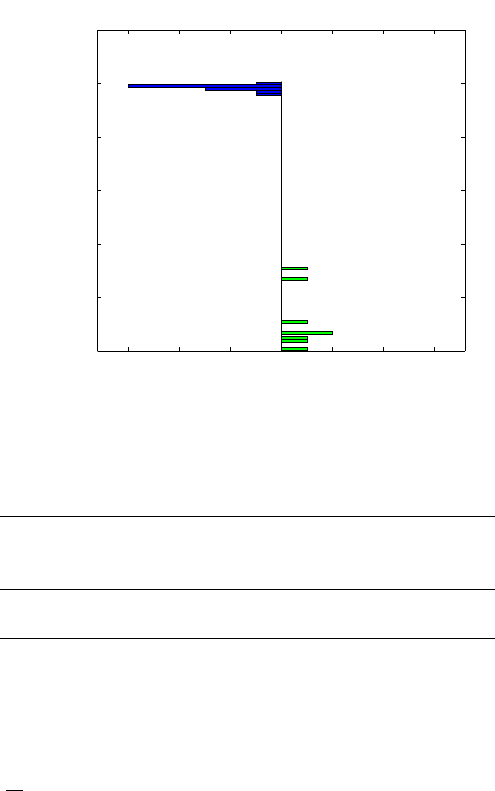
histograms (Fig. 10.2).

6 4 2 0 2 4 6

2.3

2.31

Fig. 10.2 Back-to-back histogram of Rayleigh’s measurements. Measurements from the air

are given on the left-hand side, while the measurements obtained from chemicals are on the

right.

From air 2.31035 2.31026 2.31024 2.31012

2.31027 2.31017 2.30986 2.31010

2.31001 2.31024 2.31010 2.31028

From chemicals 2.30143 2.29890 2.29816 2.30182

2.29869 2.29940 2.29849 2.29889

Assume that measurements are normal with means µ

and µ

and vari-

ances

and σ

, respectively.

Using WinBUGS and noninformative priors on the normal parameters,

ﬁnd 95% credible sets for

(a)

θ =µ

−µ

−0.01 and

(b)

ρ =

ρ >1.

10.4 Two Variances 377

We are particularly interested in (b) and (c) since Fig. 10.2 indicates that

the variability in the measurements obtained from chemicals is much higher

than in measurements obtained from the air.

The WinBUGS ﬁle

argon.odc solves (a)–(c).

#Discovery of Argon

model{

for(i in 1:n1) {

fromair[i] ~ dnorm(mu1, prec1)

}

for (j in 1:n2){

fromchem[j] ~ dnorm(mu2, prec2)

}

mu1 ~ dflat()

mu2 ~ dflat()

prec1 ~ dgamma(0.0001, 0.0001)

prec2 ~ dgamma(0.0001, 0.0001)

theta <- mu1 - mu2 - 0.01

sig2air <- 1/prec1

sig2chem <- 1/prec2

rho <- sig2chem/sig2air

ph1 <- step(rho - 1)

}

DATA

list(n1=12, n2 = 8,

fromair = c(2.31035, 2.31026, 2.31024, 2.31012, 2.31027,

2.31017, 2.30986, 2.31010, 2.31001,

2.31024, 2.31010, 2.31028),

fromchem = c(2.30143, 2.29890, 2.29816, 2.30182,

2.29869, 2.29940,

2.29849, 2.29889) )

INITS

list(mu1 = 0, mu2 = 0, prec1 = 10, prec2 = 10)

mean sd MC error val2.5pc median val97.5pc start sample

ph1 0.786 0.4101 4.473E-4 0.0 1.0 1.0 1001 1000000

rho 2.347 2.333 0.002684 0.4456 1.736 7.925 1001 1000000

theta 6.971E-4 0.002683 2.584E-6 –0.004626 6.983E-4 0.006017 1001 1000000

It is instructive to compare a frequentist test for the variance ratio with

WinBUGS output. The statistic F

= s

=0.0099 is strongly signiﬁcant with

a p-value of the order 10

−9

. At the same time, the posterior probability of ρ >1,

a Bayesian equivalent to the F test, is only 0.786. The posterior probability

ρ ≤ 1 is 0.214. Also, the 95% credible set for ρ contains 1. Even though a

Bayesian would favor the hypothesis

ρ > 1, the evidence against ρ ≤ 0 is not

as strong as in the classical approach.

378 10 Two Samples

10.5 Comparing Two Proportions

Comparing two population proportions is arguably one of the most important

tasks in statistical practice. For example, statistical support in clinical tri-

als for new drugs, procedures, or medical devices almost always contains tests

and conﬁdence intervals involving two proportions: proportions of positive out-

comes in control and treatment groups, proportions of readings within toler-

ance limits for proposed and currently approved medical devices, or propor-

tions of cancer patients for which new and old treatment regimes manifested

drug toxicity, to list just a few.

Sample proportions involve binomial distributions, and if sample sizes are

not too small, the CLT implies their approximate normality.

Let X

∼ B in(n

, p

) and X

∼ B in(n

, p

) be the observed numbers of

“events” and

and

be the sample proportions. Then the difference

−

= X

− X

has an approximately normal distribution (when n

and

are not too small, say, >20) with mean p

−p

and variance p

(1 − p

)/n

(1 − p

)/n

A Wald-type conﬁdence interval can be constructed using this normal ap-

proximation. Speciﬁcally, the (1

−α)100% conﬁdence interval for the population

proportion difference p

− p

−

−z

1−α/2

(1 −

)

(1 −

)

−

1−α/2

(1 −

)

(1 −

)

In testing H

: p

= p

against one of the alternatives, the test statistic is

−

p(1

−

p(1

−

)

where

is the pooled sample proportion. The pooled sample proportion is used since

under H

the population proportions coincide and this common parameter

should be estimated by all available data. By the CLT, the statistic Z has an

approximately standard normal

N (0,1) distribution.