Anderson D.R., Sweeney D.J., Williams T.A. Essentials of Statistics for Business and Economics
Подождите немного. Документ загружается.


12.3 Coefficient of Determination 505
a. Compute SST, SSR, and SSE.
b. Compute the coefficient of determination r
2
. Comment on the goodness of fit.
c. What is the value of the sample correlation coefficient?
20. Consumer Reports provided extensive testing and ratings for more than 100 HDTVs. An
overall score, based primarily on picture quality, was developed for each model. In
general, a higher overall score indicates better performance. The following data show the
price and overall score for the ten 42-inch plasma televisions (Consumer Reports, March
2006).
a. Use these data to develop an estimated regression equation that could be used to
estimate the overall score for a 42-inch plasma television given the price.
b. Compute r
2
. Did the estimated regression equation provide a good fit?
c. Estimate the overall score for a 42-inch plasma television with a price of $3200.
21. An important application of regression analysis in accounting is in the estimation of cost.
By collecting data on volume and cost and using the least squares method to develop an
estimated regression equation relating volume and cost, an accountant can estimate the cost
associated with a particular manufacturing volume. Consider the following sample of pro-
duction volumes and total cost data for a manufacturing operation.
a. Use these data to develop an estimated regression equation that could be used to
predict the total cost for a given production volume.
b. What is the variable cost per unit produced?
c. Compute the coefficient of determination. What percentage of the variation in total
cost can be explained by production volume?
d. The company’s production schedule shows 500 units must be produced next month.
What is the estimated total cost for this operation?
22. Refer to exercise 5, where the following data were used to investigate whether higher prices
are generally associated with higher ratings for elliptical trainers (Consumer Reports,
February 2008).
Brand Price Score
Dell 2800 62
Hisense 2800 53
Hitachi 2700 44
JVC 3500 50
LG 3300 54
Maxent 2000 39
Panasonic 4000 66
Phillips 3000 55
Proview 2500 34
Samsung 3000 39
Production Volume (units) Total Cost ($)
400 4000
450 5000
550 5400
600 5900
700 6400
750 7000
file
WEB
PlasmaTV
CH012.qxd 8/16/10 6:59 PM Page 505
Copyright 2010 Cengage Learning. All Rights Reserved. May not be copied, scanned, or duplicated, in whole or in part. Due to electronic rights, some third party content may be suppressed from the eBook and/or eChapter(s).
Editorial review has deemed that any suppressed content does not materially affect the overall learning experience. Cengage Learning reserves the right to remove additional content at any time if subsequent rights restrictions require it.

506 Chapter 12 Simple Linear Regression
Brand and Model Price ($) Rating
Precor 5.31 3700 87
Keys Fitness CG2 2500 84
Octane Fitness Q37e 2800 82
LifeFitness X1 Basic 1900 74
NordicTrack AudioStrider 990 1000 73
Schwinn 430 800 69
Vision Fitness X6100 1700 68
ProForm XP 520 Razor 600 55
file
WEB
Ellipticals
With x price ($) and y rating, the estimated regression equation is 58.158 .008449x.
For these data, SSE 173.88.
a. Compute the coefficient of determination
r
2
.
b. Did the estimated regression equation provide a good fit? Explain.
c. What is the value of the sample correlation coefficient? Does it reflect a strong or weak
relationship between price and rating?
12.4 Model Assumptions
In conducting a regression analysis, we begin by making an assumption about the appro-
priate model for the relationship between the dependent and independent variable(s). For
the case of simple linear regression, the assumed regression model is
y 
0

1
x
Then the least squares method is used to develop values for b
0
and b
1
, the estimates of the
model parameters β
0
and β
1
, respectively. The resulting estimated regression equation is
We saw that the value of the coefficient of determination (r
2
) is a measure of the goodness
of fit of the estimated regression equation. However, even with a large value of r
2
, the es-
timated regression equation should not be used until further analysis of the appropriateness
of the assumed model has been conducted. An important step in determining whether the
assumed model is appropriate involves testing for the significance of the relationship. The
tests of significance in regression analysis are based on the following assumptions about
the error term ⑀.
y
ˆ
b
0
b
1
x
y
ˆ
ASSUMPTIONS ABOUT THE ERROR TERM ⑀ IN THE REGRESSION MODEL
y 
0

1
x
1. The error term ⑀ is a random variable with a mean or expected value of zero;
that is, E(⑀) 0.
Implication: β
0
and β
1
are constants, therefore E(β
0
) β
0
and E(β
1
) β
1
;
thus, for a given value of x, the expected value of y is
(12.14)E( y) β
0
β
1
x
(continued)
CH012.qxd 8/16/10 6:59 PM Page 506
Copyright 2010 Cengage Learning. All Rights Reserved. May not be copied, scanned, or duplicated, in whole or in part. Due to electronic rights, some third party content may be suppressed from the eBook and/or eChapter(s).
Editorial review has deemed that any suppressed content does not materially affect the overall learning experience. Cengage Learning reserves the right to remove additional content at any time if subsequent rights restrictions require it.
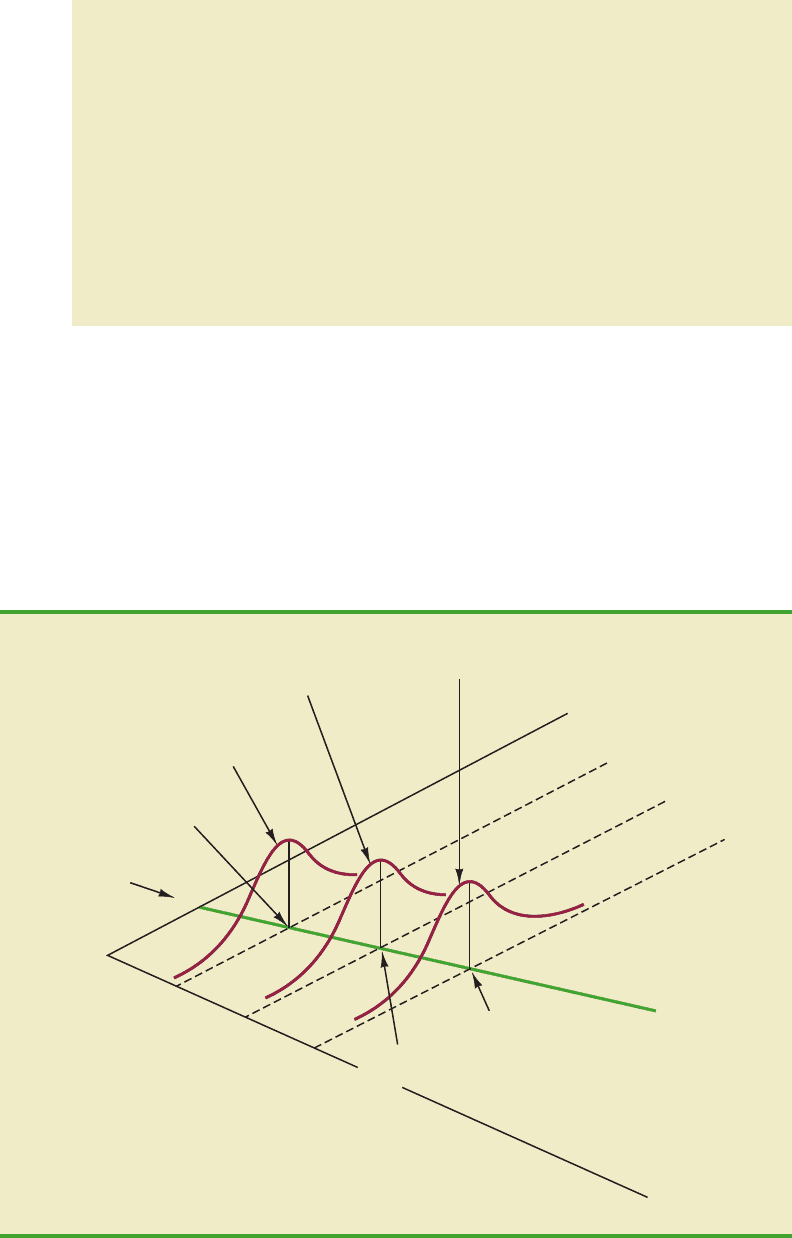
Figure 12.6 illustrates the model assumptions and their implications; note that in this
graphical interpretation, the value of E(y) changes according to the specific value of x con-
sidered. However, regardless of the x value, the probability distribution of ⑀ and hence the
probability distributions of y are normally distributed, each with the same variance. The
specific value of the error ⑀ at any particular point depends on whether the actual value of
y is greater than or less than E(y).
At this point, we must keep in mind that we are also making an assumption or hypothe-
sis about the form of the relationship between x and y. That is, we assume that a straight
12.4 Model Assumptions 507
As we indicated previously, equation (12.14) is referred to as the regression
equation.
2. The variance of ⑀, denoted by σ
2
, is the same for all values of x.
Implication: The variance of y about the regression line equals σ
2
and is the
same for all values of x.
3. The values of ⑀ are independent.
Implication:The value of ⑀ for a particular value of xis not related to the value
of ⑀ for any other value of x; thus, the value of y for a particular value of x is
not related to the value of y for any other value of x.
4. The error term ⑀ is a normally distributed random variable.
Implication: Because y is a linear function of ⑀, y is also a normally distrib-
uted random variable.
E(y) when
x = 30
x = 30
x = 20
x = 10
x
= 0
Distribution of
y at x = 30
Distribution of
y at x = 20
Distribution of
y at x = 10
β
0
y
β
0
+
β
1
x
E(y) =
x
Note: The y distributions have the
same shape at each x value.
E(y) when
x = 20
E(y) when
x = 10
E(y) when
x = 0
FIGURE 12.6 ASSUMPTIONS FOR THE REGRESSION MODEL
CH012.qxd 8/16/10 6:59 PM Page 507
Copyright 2010 Cengage Learning. All Rights Reserved. May not be copied, scanned, or duplicated, in whole or in part. Due to electronic rights, some third party content may be suppressed from the eBook and/or eChapter(s).
Editorial review has deemed that any suppressed content does not materially affect the overall learning experience. Cengage Learning reserves the right to remove additional content at any time if subsequent rights restrictions require it.

508 Chapter 12 Simple Linear Regression
line represented by β
0
β
1
x is the basis for the relationship between the variables. We must
not lose sight of the fact that some other model, for instance y β
0
β
1
x
2
⑀, may turn
out to be a better model for the underlying relationship.
12.5 Testing for Significance
In a simple linear regression equation, the mean or expected value of y is a linear function
of x: E(y) β
0
β
1
x. If the value of β
1
is zero, E(y) β
0
(0)x β
0
. In this case, the
mean value of y does not depend on the value of x and hence we would conclude that x and
y are not linearly related.Alternatively, if the value of β
1
is not equal to zero, we would con-
clude that the two variables are related. Thus, to test for a significant regression relationship,
we must conduct a hypothesis test to determine whether the value of β
1
is zero. Two tests
are commonly used. Bothrequire anestimate of σ
2
, the variance of⑀ inthe regressionmodel.
Estimate of σ
2
From the regression model and its assumptions we can conclude that σ
2
, the variance of ⑀,
also represents the variance of the y values about the regression line. Recall that the devia-
tions of the y values about the estimated regression line are called residuals. Thus, SSE, the
sum of squared residuals, is a measure of the variability of the actual observations about the
estimated regression line. The mean square error (MSE) provides the estimate of σ
2
; it is
SSE divided by its degrees of freedom.
With b
0
b
1
x
i
, SSE can be written as
Every sum of squares has associated with it a number called its degrees of freedom. Statis-
ticians have shown that SSE has n 2 degrees of freedom because two parameters (β
0
and
β
1
) must be estimated to compute SSE. Thus, the mean square error is computed by divid-
ing SSE by n 2. MSE provides an unbiased estimator of σ
2
. Because the value of MSE
provides an estimate of σ
2
, the notation s
2
is also used.
SSE 兺( y
i
y
ˆ
i
)
2
兺( y
i
b
0
b
1
x
i
)
2
y
ˆ
i
InSection12.3weshowedthatfortheArmand’sPizzaParlorsexample,SSE 1530;hence,
provides an unbiased estimate of σ
2
.
To estimate σ we take the square root of s
2
. The resulting value, s, is referred to as the
standard error of the estimate.
s
2
MSE
1530
8
191.25
MEAN SQUARE ERROR (ESTIMATE OF σ
2
)
(12.15)
s
2
MSE
SSE
n 2
STANDARD ERROR OF THE ESTIMATE
(12.16)s
兹
MSE
冑
SSE
n 2
CH012.qxd 8/16/10 6:59 PM Page 508
Copyright 2010 Cengage Learning. All Rights Reserved. May not be copied, scanned, or duplicated, in whole or in part. Due to electronic rights, some third party content may be suppressed from the eBook and/or eChapter(s).
Editorial review has deemed that any suppressed content does not materially affect the overall learning experience. Cengage Learning reserves the right to remove additional content at any time if subsequent rights restrictions require it.

12.5 Testing for Significance 509
For the Armand’s Pizza Parlors example, In the follow-
ing discussion, we use the standard error of the estimate in the tests for a significant rela-
tionship between x and y.
t Test
The simple linear regression model is y β
0
β
1
x ⑀. If x and y are linearly related, we
must have β
1
0. The purpose of the t test is to see whether we can conclude that β
1
0.
We will use the sample data to test the following hypotheses about the parameter β
1
.
If H
0
is rejected, we will conclude that β
1
0 and that a statistically significant rela-
tionship exists between the two variables. However, if H
0
cannot be rejected, we will have
insufficient evidence to conclude that a significant relationship exists. The properties of
the sampling distribution of b
1
, the least squares estimator of β
1
, provide the basis for the
hypothesis test.
First, let us consider what would happen if we used a different random sample for the
same regression study. For example, suppose that Armand’s Pizza Parlors used the sales
records of a different sample of 10 restaurants. A regression analysis of this new sample
might result in an estimated regression equation similar to our previous estimated regres-
sion equation 60 5x. However, it is doubtful that we would obtain exactly the same
equation (with an intercept of exactly 60 and a slope of exactly 5). Indeed, b
0
and b
1
, the
least squares estimators, are sample statistics with their own sampling distributions. The
properties of the sampling distribution of b
1
follow.
y
ˆ
H
0
:
H
a
:
β
1
0
β
1
0
s
兹
MSE
兹
191.25 13.829.
Note that the expected value of b
1
is equal to β
1
, so b
1
is an unbiased estimator of β
1
.
Because we do not know the value of σ, we develop an estimate of , denoted , by
estimating σ with s in equation (12.17). Thus, we obtain the following estimate of .σ
b
1
s
b
1
σ
b
1
SAMPLING DISTRIBUTION OF b
1
Expected Value
Standard Deviation
(12.17)
Distribution Form
Normal
σ
b
1
σ
兹
兺(x
i
x¯)
2
E(b
1
) β
1
ESTIMATED STANDARD DEVIATION OF b
1
(12.18)s
b
1
s
兹
兺(x
i
x¯)
2
The standard deviation of
b
1
is also referred to as the
standard error of b
1
. Thus,
provides an estimate of
the standard error of b
1
.
s
b
1
CH012.qxd 8/16/10 6:59 PM Page 509
Copyright 2010 Cengage Learning. All Rights Reserved. May not be copied, scanned, or duplicated, in whole or in part. Due to electronic rights, some third party content may be suppressed from the eBook and/or eChapter(s).
Editorial review has deemed that any suppressed content does not materially affect the overall learning experience. Cengage Learning reserves the right to remove additional content at any time if subsequent rights restrictions require it.

510 Chapter 12 Simple Linear Regression
For Armand’s Pizza Parlors, s 13.829. Hence, using 兺(x
i
)
2
568 as shown in Table 12.2,
we have
as the estimated standard deviation of b
1
.
The t test for a significant relationship is based on the fact that the test statistic
follows a t distribution with n 2 degrees of freedom. If the null hypothesis is true, then
β
1
0 and t b
1
/.s
b
1
b
1
β
1
s
b
1
s
b
1
13.829
兹
568
.5803
x¯
t TEST FOR SIGNIFICANCE IN SIMPLE LINEAR REGRESSION
TEST STATISTIC
(12.19)
REJECTION RULE
where t
α/2
is based on a t distribution with n 2 degrees of freedom.
p-value approach:
Critical value approach:
Reject H
0
if p-value α
Reject H
0
if t t
α/2
or if t t
α/2
t
b
1
s
b
1
H
0
:
H
a
:
β
1
0
β
1
0
Confidence Interval for β
1
The form of a confidence interval for β
1
is as follows:
b
1
t
α/2
s
b
1
Let us conduct this test of significance for Armand’s Pizza Parlors at the α .01 level
of significance. The test statistic is
The t distribution table shows that with n 2 10 2 8 degrees of freedom, t 3.355
provides an area of .005 in the upper tail.Thus, the area in the upper tail of the t distribution
corresponding to the test statistic t 8.62 must be less than .005. Because this test is a two-
tailed test, we double this value to conclude that the p-value associated with t 8.62 must
be less than 2(.005) .01. Excel or Minitab show the p-value .000. Because the p-value
is less than α .01, we reject H
0
and conclude that β
1
is not equal to zero. This evidence is
sufficient to conclude that a significant relationship exists between student population and
quarterly sales.Asummary of the t test for significance in simple linear regression follows.
t
b
1
s
b
1
5
.5803
8.62
Appendixes 12.3 and 12.4
show how Minitab and
Excel can be used to
compute the p-value.
CH012.qxd 8/16/10 6:59 PM Page 510
Copyright 2010 Cengage Learning. All Rights Reserved. May not be copied, scanned, or duplicated, in whole or in part. Due to electronic rights, some third party content may be suppressed from the eBook and/or eChapter(s).
Editorial review has deemed that any suppressed content does not materially affect the overall learning experience. Cengage Learning reserves the right to remove additional content at any time if subsequent rights restrictions require it.

12.5 Testing for Significance 511
The point estimator is b
1
and the margin of error is t
α/2
. The confidence coefficient asso-s
b
1
ciated with this interval is 1 α, and t
α/2
is the t value providing an area of α/2 in the up-
per tail of a t distribution with n 2 degrees of freedom. For example, suppose that we
wanted to develop a 99% confidence interval estimate of β
1
for Armand’s Pizza Parlors.
From Table 2 of Appendix B we find that the t value corresponding to α .01 and
n 2 10 2 8 degrees of freedom is t
.005
3.355. Thus, the 99% confidence interval
estimate of β
1
is
or 3.05 to 6.95.
In using the t test for significance, the hypotheses tested were
At the α .01 level of significance, we can use the 99% confidence interval as an alterna-
tive for drawing the hypothesis testing conclusion for the Armand’s data. Because 0, the hy-
pothesized value of β
1
, is not included in the confidence interval (3.05 to 6.95), we can reject
H
0
and conclude that a significant statistical relationship exists between the size of the stu-
dent population and quarterly sales. In general, a confidence interval can be used to test any
two-sided hypothesis about β
1
. If the hypothesized value of β
1
is contained in the confi-
dence interval, do not reject H
0
. Otherwise, reject H
0
.
F Test
An F test, based on the F probability distribution, can also be used to test for significance
in regression. With only one independent variable, the F test will provide the same conclu-
sion as the t test; that is, if the t test indicates β
1
0 and hence a significant relationship,
the F test will also indicate a significant relationship. But with more than one independent
variable, only the F test can be used to test for an overall significant relationship.
The logic behind the use of the F test for determining whether the regression relation-
ship is statistically significant is based on the development of two independent estimates of
σ
2
. We explained how MSE provides an estimate of σ
2
. If the null hypothesis H
0
: β
1
0 is
true, the sum of squares due to regression, SSR, divided by its degrees of freedom provides
another independent estimate of σ
2
. This estimate is called the mean square due to regres-
sion, or simply the mean square regression, and is denoted MSR. In general,
For the models we consider in this text, the regression degrees of freedom is always
equal to the number of independent variables in the model:
(12.20)
Because we consider only regression models with one independent variable in this chapter, we
have MSR SSR/1 SSR. Hence, for Armand’s Pizza Parlors, MSR SSR 14,200.
If the null hypothesis (H
0
: β
1
0) is true, MSR and MSE are two independent estimates
of σ
2
and the sampling distribution of MSR/MSE follows an F distribution with numerator
MSR
SSR
Number of independent variables
MSR
SSR
Regression degrees of freedom
H
0
:
H
a
:
β
1
0
β
1
0
b
1
t
α/2
s
b
1
5
3.355(.5803) 5
1.95
CH012.qxd 8/16/10 6:59 PM Page 511
Copyright 2010 Cengage Learning. All Rights Reserved. May not be copied, scanned, or duplicated, in whole or in part. Due to electronic rights, some third party content may be suppressed from the eBook and/or eChapter(s).
Editorial review has deemed that any suppressed content does not materially affect the overall learning experience. Cengage Learning reserves the right to remove additional content at any time if subsequent rights restrictions require it.

512 Chapter 12 Simple Linear Regression
degrees of freedom equal to one and denominator degrees of freedom equal to n 2. There-
fore, when β
1
0, the value of MSR/MSE should be close to 1. However, if the null hy-
pothesis is false (β
1
0), MSR will overestimate σ
2
and the value of MSR/MSE will be
inflated; thus, large values of MSR/MSE lead to the rejection of H
0
and the conclusion that
the relationship between x and y is statistically significant.
Let us conduct the F test for the Armand’s Pizza Parlors example. The test statistic is
The F distribution table (Table 4 ofAppendix B) shows that with one degree of freedom in
the numerator and n 2 10 2 8 degrees of freedom in the denominator, F 11.26
provides an area of .01 in the upper tail. Thus, the area in the upper tail of the F distribution
corresponding to the test statistic F 74.25 must be less than .01. Thus, we conclude that
the p-value must be less than .01. Excel or Minitab show the p-value .000. Because the
p-value is less than α .01, we reject H
0
and conclude that a significant relationship exists
between the size of the student population and quarterly sales. Asummary of the F test for
significance in simple linear regression follows.
F
MSR
MSE
14,200
191.25
74.25
In Chapter 10 we covered analysis of variance (
ANOVA) and showed how an ANOVA
tablecould be used to provide a convenient summary of the computational aspects of analy-
sis of variance. A similar ANOVA table can be used to summarize the results of the F test
for significance in regression. Table 12.5 is the general form of the ANOVA table for simple
linear regression. Table 12.6 is the ANOVA table with the F test computations performed
for Armand’s Pizza Parlors. Regression, Error, and Total are the labels for the three sources
of variation, with SSR, SSE, and SST appearing as the corresponding sum of squares in col-
umn 2. The degrees of freedom, 1 for SSR, n 2 for SSE, and n 1 for SST, are shown in
column 3. Column 4 contains the values of MSR and MSE, column 5 contains the value of
F MSR/MSE, and column 6 contains the p-value corresponding to the F value in column 5.
Almost all computer printouts of regression analysis include an ANOVA table summary of
the F test for significance.
The F test and the t test
provide identical results for
simple linear regression.
F TEST FOR SIGNIFICANCE IN SIMPLE LINEAR REGRESSION
TEST STATISTIC
(12.21)
REJECTION RULE
where F
α
is based on an F distribution with 1 degree of freedom in the numerator and
n 2 degrees of freedom in the denominator.
p-value approach:
Critical value approach:
Reject H
0
if p-value α
Reject H
0
if F F
α
F
MSR
MSE
H
0
:
H
a
:
β
1
0
β
1
0
If H
0
is false, MSE still
provides an unbiased
estimate of σ
2
and MSR
overestimates σ
2
. If H
0
is
true, both MSE and MSR
provide unbiased estimates
of σ
2
; in this case the value
of MSR/MSE should be
close to 1.
CH012.qxd 8/16/10 6:59 PM Page 512
Copyright 2010 Cengage Learning. All Rights Reserved. May not be copied, scanned, or duplicated, in whole or in part. Due to electronic rights, some third party content may be suppressed from the eBook and/or eChapter(s).
Editorial review has deemed that any suppressed content does not materially affect the overall learning experience. Cengage Learning reserves the right to remove additional content at any time if subsequent rights restrictions require it.

12.5 Testing for Significance 513
Some Cautions About the Interpretation
of Significance Tests
Rejecting the null hypothesis H
0
: β
1
0 and concluding that the relationship between x and
y is significant do not enable us to conclude that a cause-and-effect relationship is present
between x and y. Concluding a cause-and-effect relationship is warranted only if the ana-
lyst can provide some type of theoretical justification that the relationship is in fact causal.
In the Armand’s Pizza Parlors example, we can conclude that there is a significant rela-
tionship between the size of the student population x and quarterly sales y; moreover, the
estimated regression equation 60 5x provides the least squares estimate of the rela-
tionship. We cannot, however, conclude that changes in student population x cause changes
in quarterly sales y just because we identified a statistically significant relationship. The ap-
propriateness of such a cause-and-effect conclusion is left to supporting theoretical justifi-
cation and to good judgment on the part of the analyst. Armand’s managers felt that
increases in the student population were a likely cause of increased quarterly sales. Thus,
the result of the significance test enabled them to conclude that a cause-and-effect rela-
tionship was present.
In addition, just because we are able to reject H
0
: β
1
0 and demonstrate statistical sig-
nificance does not enable us to conclude that the relationship between x and y is linear. We
can state only that x and y are related and that a linear relationship explains a significant
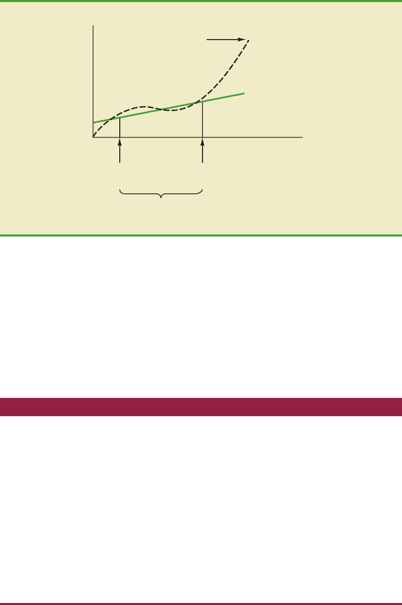
portion of the variability in y over the range of values for x observed in the sample. Fig-
ure 12.7 illustrates this situation. The test for significance calls for the rejection of the null
hypothesis H
0
: β
1
0 and leads to the conclusion that x and y are significantly related, but
the figure shows that the actual relationship between x and y is not linear. Although the
y
ˆ
Regression analysis, which
can be used to identify how
variables are associated
with one another, cannot be
used as evidence of a
cause-and-effect
relationship.
Source Sum Degrees Mean
of Variation of Squares of Freedom Square Fp-value
Regression SSR 1
Error SSE
Total SST n 1
MSE
SSE
n 2
n 2
F
MSR
MSE
MSR
SSR
1
TABLE 12.5
GENERAL FORM OF THE ANOVATABLE FOR SIMPLE
LINEAR REGRESSION
In every analysis of
variance table the total sum
of squares is the sum of the
regression sum of squares
and the error sum of
squares; in addition, the
total degrees of freedom is
the sum of the regression
degrees of freedom and the
error degrees of freedom.
Source Sum Degrees Mean
of Variation of Squares of Freedom Square Fp-value
Regression 14,200 1 .000
Error 1,530 8
Total 15,730 9
1530
8
191.25
14,200
191.25
74.25
14,200
1
14,200
TABLE 12.6
ANOVA TABLE FOR THE ARMAND’S PIZZA PARLORS PROBLEM
CH012.qxd 8/16/10 6:59 PM Page 513
Copyright 2010 Cengage Learning. All Rights Reserved. May not be copied, scanned, or duplicated, in whole or in part. Due to electronic rights, some third party content may be suppressed from the eBook and/or eChapter(s).
Editorial review has deemed that any suppressed content does not materially affect the overall learning experience. Cengage Learning reserves the right to remove additional content at any time if subsequent rights restrictions require it.
514 Chapter 12 Simple Linear Regression
linear approximation provided by b
0
b
1
x is good over the range of x values observed
in the sample, it becomes poor for x values outside that range.
Given a significant relationship, we should feel confident in using the estimated re-
gression equation for predictions corresponding to x values within the range of the x values
observed in the sample. For Armand’s Pizza Parlors, this range corresponds to values of x
between 2 and 26. Unless other reasons indicate that the model is valid beyond this range,
predictions outside the range of the independent variable should be made with caution. For
Armand’s Pizza Parlors, because the regression relationship has been found significant at
the .01 level, we should feel confident using it to predict sales for restaurants where the
associated student population is between 2000 and 26,000.
y
ˆ
y = b
0
+ b
1
x
^
Actual
relationship
y
Smallest
x value
Largest
x value
Range of x
values observed
x
FIGURE 12.7 EXAMPLE OF A LINEAR APPROXIMATION OF A NONLINEAR
RELATIONSHIP
NOTES AND COMMENTS
1. The assumptions made about the error term
(Section 12.4) are what allow the tests of statis-
tical significance in this section. The properties
of the sampling distribution of b
1
and the sub-
sequent t and F tests follow directly from these
assumptions.
2. Do not confuse statistical significance with
practical significance. With very large sample
sizes, statistically significant results can be ob-
tained for small values of b
1
; in such cases, one
must exercise care in concluding that the rela-
tionship has practical significance.
3. A test of significance for a linear relationship
between x and y can also be performed by using
the sample correlation coefficient r
xy
. With
xy
denoting the population correlation coefficient,
the hypotheses are as follows.
A significant relationship can be concluded if H
0
is rejected. The details of this test are provided
in more advanced texts. However, the t and F
tests presented previously in this section give
the same result as the test for significance using
the correlation coefficient. Conducting a test for
significance using the correlation coefficient
therefore is not necessary if a t or F test has
already been conducted.
H
0
:
H
a
:
r
xy
0
r
xy
0
CH012.qxd 8/16/10 6:59 PM Page 514
Copyright 2010 Cengage Learning. All Rights Reserved. May not be copied, scanned, or duplicated, in whole or in part. Due to electronic rights, some third party content may be suppressed from the eBook and/or eChapter(s).
Editorial review has deemed that any suppressed content does not materially affect the overall learning experience. Cengage Learning reserves the right to remove additional content at any time if subsequent rights restrictions require it.