Andrews Dawid G. An Introduction to Atmospheric Physics

Подождите немного. Документ загружается.

209 The radiative forcing due to an increase in carbon dioxide

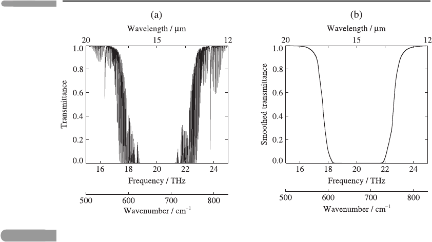
Fig. 8.5 (a) Spectrum of T

for the main absorption band of CO

, plotted against frequency ν in THz and

also against wavenumber

ν in cm

−1

and wavelength in μm, at a resolution of 0.3 GHz

(0.01 cm

−1

), based on data provided by Dr A. Dudhia. (b) A smoothed version of the same

spectrum: this is obtained by reordering the original spectrum with respect to frequency, to make

it monotonic in frequency on either side of the centre of the band. The range of variation of T

and the area under the curve are unchanged by the reordering.

smoothed spectrum, we note that, as ν increases, T

drops from 1 to 0 between about 16

and 18 THz and then rises from 0 to 1 between about 22 and 24 THz. The maximum value

max

of D(T

) will be attained at certain frequencies in these regions on the ‘ﬂanks’, or

‘wings’, of the absorption band.

Outside these regions T

equals either 1−1or0−0, i.e. it is zero; so by equation (8.27)

the change F

↑

in SOLR is also zero there. Physically, there can be no change in SOLR

at those frequencies where the troposphere is either completely transparent (optically thin)

or completely opaque (optically thick): neither of these cases is affected by an increase in

absorber density.

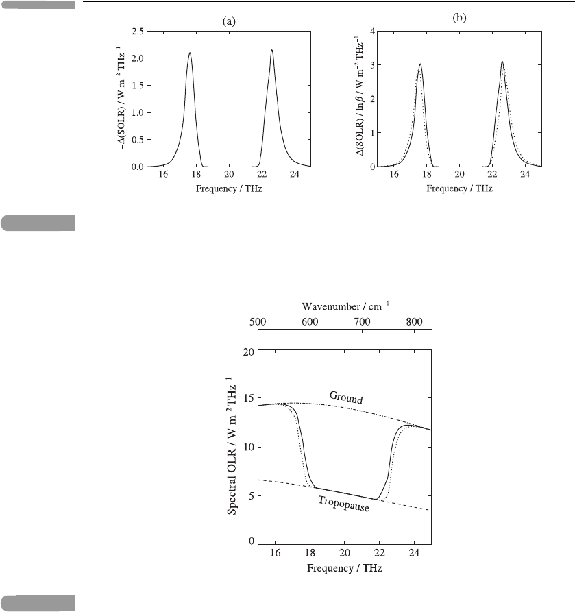
Figure 8.6(a) shows the decrease in SOLR for the case β = 2, with T

= 290 K

and T

= 225 K chosen to represent a typical observed mid-latitude upper-tropospheric

temperature. This decrease has a peak, with maximum value π(B

νg

− B

νt

max

, on each

ﬂank of the absorption band. Figure 8.6(b) shows the decrease in SOLR divided by ln β,for

β = 2 and 4; the fact that the two curves are so close together indicates that the approximate

logarithmic dependence of D

max

in equation (8.29) carries over to −F

↑

at each frequency.

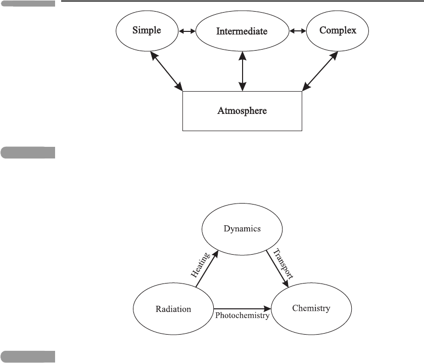
Another way of looking at this result is to plot the unperturbed SOLR, and the SOLR

under a doubling of CO

, against frequency: see Figure 8.7. Also plotted are πB

for the

surface and the troposphere (which is again given a typical observed upper-tropospheric

temperature). As expected from equation (8.25), both SOLR curves lie between the two

Planck function curves, rising to meet the surface curve outside the absorption band, and

210 Climate change

Fig. 8.6

(a) Decrease −F

↑

in SOLR given by equation (8.27) for a doubling of CO

density (β = 2), based

on the smoothed spectrum on the right of Figure 8.5,withT

= 290 K and T

= 225 K. (b)

−F

↑

/ ln β,forβ = 2 (solid) and 4 (dotted).

Fig. 8.7

Unperturbed SOLR F

↑

(solid), and the SOLR under a doubling of CO

(dotted), based on the

smoothed spectrum on the right of Figure 8.5, plotted against frequency and wavenumber. Also

shown are π B

evaluated at the surface (dot-dashed) and at the tropopause (dashed), with

= 290 K and T

= 225 K.

falling to meet the tropopause curve inside it. As CO

doubles, the SOLR decreases a little

at each wavenumber on the ﬂanks of the CO

band. The decrease from the unperturbed

case is given by the vertical distance between the two SOLR curves, and this is equal to

the function plotted in Figure 8.6(a). This decrease leads to a broadening of the ‘bite’ taken

out of the surface Planck function curve: see Pierrehumbert (2010).

211 The radiative forcing due to an increase in carbon dioxide

The ﬁnal stage in the calculation of the radiative forcing is to integrate the spectral

results over frequency, i.e. to calculate the areas under the curves in Figure 8.6(b).

(See

Problem 8.9.) The fact that these areas depend only weakly on β shows that the approximate

logarithmic dependence carries over to the radiative forcing F, which therefore takes the

form

F =−



∞

F

↑

dν ≈ A ln β, (8.30)

where A is a constant, in agreement with the form of equation (8.24). Note that the

logarithmic dependence does not depend on the detailed structure of the spectral lines, but

just on the fact that the tropospheric transmittance varies rapidly in frequency between 0 and

1 on each ﬂank of the absorption band, so that the most signiﬁcant values of the transmittance

change (almost proportional to ln β) are attained in a narrow range of frequencies there.

The integral is dominated by contributions from frequencies in these ﬂank regions.

For comparison with Section 8.2, it is convenient to put U = ln ρ

,whereρ

= ρ

(0)

is the CO

density at the ground. The change from ρ

to βρ

then corresponds to the ﬁnite

change U = ln β,soequation (8.30) gives F ≈ A U.Thisimpliesthatequation (8.7)

holds without the ‘small perturbation’ assumption, given ∂Q/∂U = A.

The CO

case should be contrasted with that of absorbers such as the chloroﬂuorocarbons,

which are optically thin at all frequencies, so that T

is always close to 1 (i.e. it is always

close to the right-hand end of the range shown in Figure 8.4), and D

max

is never attained

at any ν. In this case we can show (e.g. by putting T

= 1 − A

,whereA

 1) that

D(T

) ∼ (β − 1)(1 − T

). Therefore for such absorbers the radiative forcing is linear, not

logarithmic, in β: this is conﬁrmed by detailed calculations.

Of course, our simple slab model is an extremely crude representation of the real

troposphere. However, it can be extended to a multi-level model in which the temperature

follows a speciﬁed lapse rate; the argument that we have used is applied at each level

within the troposphere, and then a vertical integral performed. Approximate logarithmic

dependence of the SOLR at each frequency is found, and essentially the same results follow.

Further reading

A good introduction to the physics of climate change is given by Hartmann (1994). The

advanced but readable book by Pierrehumbert (2010) covers the material of this chapter

in more detail, and goes much further – including, for example, the physics of climate

change in the Earth’s distant past and on other planets. The Fourth Assessment Report of

the Intergovernmental Panel on Climate Change, Working Group I (Solomon et al. (2007)),

gives a wealth of up-to-date information on climate change and the physical processes

contributing to it. Houghton (2009) provides an authoritative overview of the current

This is almost identical to integrating the unsmoothed functions, since the smoothing just reorders them with

respect to frequency. The Planck function is not reordered; however, it only varies slowly with frequency. Note

also that other CO

absorption bands are present, as shown by Figure 3.14, but these are less important because

is much smaller for the frequencies and temperatures involved.

212 Climate change

understanding of the science of climate change and its impacts on human society. See Bates

(2007) for a thorough discussion of the concept of ‘climate feedback’. The paper by Myhre

et al. (1998) provides detailed calculations of the radiative forcing due to changes in CO

and other greenhouse gases.

Problems

Problem 8.1 Consider a model troposphere in the form of a thin slab at a temperature

above a warmer black surface at temperature T

. (This system need not be in radiative

equilibrium, i.e. non-radiative heat transfers could occur.) Suppose that the troposphere

contains a greenhouse gas whose absorption coefﬁcient is independent of frequency in the

infra-red (this is called a ‘grey’ absorber) and whose infra-red transmittance is T . Show

that the upward irradiance above the troposphere is given by

↑

= T σ T

+ (1 − T )σ T

, (8.31)

where σ is Boltzmann’s constant.

Assuming that F

↑

balances the unreﬂected incoming solar irradiance F

= 240 W m

−2

and given that the tropospheric temperature T

= 245 K, ﬁnd the surface temperature T

for

T = 0.1, 0.2 and 0.3. Show that the ‘greenhouse effect’ of the gas, deﬁned as σ T

−F

,is

proportional to T

−1

−1 and evaluate it in each case. Repeat the calculations for T

= 225 K.

Comment on the implication of your answers.

Problem 8.2 Suppose that the troposphere in the previous problem contains two green-

house gases that are both grey absorbers and whose infra-red transmittances are T

and

, both less than 1. Show that their combined transmittance is T

. Hence show that

the greenhouse effect of the combination of gases is not equal to the sum of their separate

greenhouse effects, except (approximately) when both gases are optically thin, i.e. when

and T

are both close to 1. (Hint for last part: put T

= 1 −A

,whereA

is small, etc.)

Problem 8.3 Find an expression for the response of the EBM (8.8) to the exponentially

decaying pulse forcing (8.17). Verify the plot of the time-dependence of T



in Figure 8.2(c),

given τ = 30 years and t

= 1.5 years. What scaling is used for T



in that ﬁgure? Find the

maximum negative temperature response, given F

=−2Wm

−2

Problem 8.4 Find expressions for the response of the EBM (8.8) to the sinusoidal solar

cycle forcing (8.18), ignoring transients, i.e. ﬁnd T



in the form a sin(ωt − φ),wherethe

amplitude a and phase lag φ are to be obtained. (Hint: it may be helpful to use complex

exponentials.) What are the values of the amplitude and the phase lag, given τ = 30 years

and F

= 0.12 W m

−2

A hypothetical ‘equilibrium response’ to the forcing can be deﬁned as the solution for

the case when the time-derivative on the left of equation (8.8) is ignored. Evaluate the ratio

213 Problems

of a to the amplitude of the equilibrium response, given τ as above. Sketch the forcing, the

full solution and the equilibrium solution on the same time axis.

Problem 8.5

1. Using the formula given in equation (8.24), evaluate the radiative forcing F

2×CO

associated with a doubling of CO

2. Assuming an increase in CO

concentration of 0.5% per year, evaluate the constant

γ = dF/dt in equation (8.15). If this rate were sustained, how many years would it take

for the concentration to double? How long would it take for the volume mixing ratio to

increase from a recent value of 385 ppmv (cf. Table 2.1) to 550 ppmv (approximately

double the pre-industrial value)?

3. Assuming that the only feedback process is black-body feedback, evaluate the climate

sensitivity under an instantaneous doubling of CO

. Given that the climate system has

a heat capacity C per unit horizontal area of 1 GJ K

−1

−2

, evaluate the corresponding

feedback response time (FRT) τ .

4. The climate sensitivity in a complex climate-forecast model is in fact found to be

3 K under an instantaneous doubling of CO

. What value of the feedback param-

eter α does this correspond to? Assuming the same value of C as above, evaluate

the FRT in this case. Comment on the effects of non-black-body feedbacks in

this model.

5. Now suppose that errors in the climate-forecast model imply that the value of α obtained

above is uncertain to within ±50%. What are the corresponding ranges of uncertainty

of climate sensitivity and FRT? Comment on the distribution of these ranges about the

values established in the previous paragraph.

Problem 8.6 For the ‘ramp-ﬂat’ model of Section 8.3.1, show that the ratio of the

equilibrium temperature perturbation to that at time t

is a function of x = t

/τ only. Show

that this function is large for small x and tends to 1 for large x, and give a rough sketch of

it. Conﬁrm that the shape of this function agrees with the results plotted in Figure 8.3.

For the three values of τ used in Figure 8.3, ﬁnd the times at which T



reaches 90% and

99%, respectively, of its equilibrium value T

eqm

Problem 8.7 Consider a simple energy balance model including ice-albedo feedback, in

which the Earth’s albedo A varies strongly with the amount of ice cover: represent this by

allowing A to vary with temperature as follows:

A = 0.6 for T ≤ 265 K,

A = 0.3 for T ≥ 275 K,

A = 0.45 + 0.03 × (270 K − T) for 265 K ≤ T ≤ 275 K.

Hence modify equation (8.2) for F

↓

appropriately; assume F

↑

(T) = 0.6 σ T

,wherethe

emissivity factor 0.6 is a simple representation of the greenhouse effect.

214 Climate change

1. Give a brief physical explanation of the formula for A(T).

2. Show that this model has equilibrium (steady-state) solutions for a temperature T

265 K (‘snowball Earth’) and a temperature T

> 275 K, and evaluate T

and T

.Draw

asketchofF

↓

(T) and F

↑

(T) as functions of T. Show from your sketch that there is also

an equilibrium temperature T

between 265 and 275 K. (Do not evaluate T

: it is in fact

about 269 K).

3. Find an expression for the feedback parameter α =−dQ/dT for this model, where

Q(T) = F

↓

− F

↑

. From your sketch determine the sign of α at each equilibrium

temperature, and hence infer whether each equilibrium is stable or unstable. Comment

on the concept of ‘ice-albedo feedback’ in this model.

Problem 8.8 Given the function D deﬁned by equation (8.28), show that its maximum

value for each β is

max

= β

−1/(β−1)

− β

−β/(β−1)

Now show that D

max

can be written in terms of u ≡ ln β as

max

= exp



−u

− 1



− exp



−u

1 − e

−u



Verify that D

max

is an odd function of u. By expanding to the ﬁrst power in u show that

max

∼

ln β as u → 0 , i.e. as β → 1. (8.32)

Without detailed calculation show that the next term in the expansion must be of order u

Verify that the approximation (8.29) for D

max

is about 8% too large at β = 4.

Problem 8.9 Use Figure 8.6 to obtain a rough estimate of the coefﬁcient A of ln β in

equation (8.30) for the radiative forcing for CO

Atmospheric modelling

This chapter is a short introduction to the use of models in atmospheric research and

forecasting. In Section 9.1 we explain how a hierarchy of models – simple, intermediate and

complex – can be used for gaining understanding of atmospheric behaviour and interpreting

atmospheric data. In Section 9.2 we give brief details of the numerical methods used in the

more complex theoretical models, while in Section 9.3 we outline the use of these models

for forecasting and other purposes. In Section 9.4 we describe an example of a class of

laboratory models of the atmosphere. Finally, in Section 9.5,wegivesomeexamplesof

atmospheric phenomena that arise from interactions between basic physical processes and

that can be elucidated only with the aid of models of intermediate complexity.

9.1 The hierarchy of models

The basic philosophy of atmospheric modelling was outlined in Section 1.2.Itwas

mentioned there that a hierarchy of models, from simple to complex, must be used for under-

standing and predicting atmospheric behaviour; this hierarchy is illustrated in Figure 9.1.

The simple models (‘back-of-the-envelope’ or ‘toy’ models) involve a minimum number

of physical components and are described by straightforward mathematical equations that

can usually be solved analytically. These models provide basic physical intuition: most of

the models considered earlier in this book are of this type. The intermediate models involve

a small number of physical components but usually require a computer for solution of the

mathematical equations. Simple and intermediate models can provide valuable conceptual

pictures of atmospheric processes, but do not usually give accurate simulations of actual

atmospheric behaviour. The complex models (often called general circulation models

or GCMs) contain mathematical representations of a large number of physical processes.

These are the models that are used when accurate simulations are required.

Each type of model is motivated by atmospheric observations and each may help us

understand some aspect of atmospheric behaviour. The physical intuition provided by the

simplest models helps us interpret the intermediate models and the intermediate models

help us interpret the complex models. When a complex model fails to produce a reasonable

simulation of observed atmospheric behaviour, it may be necessary to use an intermediate

model (perhaps a ‘stripped-down’ version of the complex model) to ﬁnd the cause.

The types of physical process that can be included in atmospheric models fall into three

main categories, each of which has been studied in earlier chapters.

216 Atmospheric modelling

Fig. 9.1

Illustrating the use of a hierarchy of atmospheric models. Each type of model is motivated by,

and provides some insight into, atmospheric behaviour. The simpler models help us interpret the

more complex models. If a more complex model fails, a simpler model may help us to locate

the cause.

Fig. 9.2

Illustrating some of the interactions among dynamics, radiation and chemistry in the

atmosphere; see the text for details.

• Dynamical processes, including those parts of thermodynamics associated with the First

Law. These were introduced in Chapters 4 and 5.

• Radiation: this was introduced in Chapter 3, and some of its consequences for climate

change were explored in Chapter 8.

• Chemistry: some aspects of this were introduced in Chapter 6.

These three categories interact in complex ways in the atmosphere, as is partly illustrated

in Figure 9.2. Transport by dynamical processes carries chemicals from one part of the

atmosphere to another, for example vertically from ground level to the stratosphere, or

horizontally from the industrialised Northern Hemisphere to Antarctica; see Section 6.6.

The heating due to absorption of solar ultra-violet radiation by ozone may drive dynamical

processes. Solar radiation may be energetic enough to disrupt chemical bonds, leading

to photochemical reactions. In general, models incorporating even a few of these inter-

actions will be too complicated for simple analysis and so will be of ‘intermediate’ or

‘complex’ type.

217 Numerical methods

9.2 Numerical methods

As mentioned in Section 9.1, intermediate and complex models require us to solve the

mathematical equations describing the physics by means of computers. This is not an easy

task and may require extremely careful and efﬁcient computer programming and huge

computer codes. In this section we describe some of the basic principles involved.

The equations describing the dynamics are generally partial differential equations, invol-

ving differentiation in space and time. Consider for example the x-momentum equation;

under the approximations discussed in Section 4.7.2 this can be written

∂u

∂t

=−u

∂u

∂x

− v

∂u

∂y

− w

∂u

∂z

+ f v −

∂p

∂x

+ F

(x)

, (9.1)

by equations (4.23a) and (4.22). The physical meanings of the symbols are given in

Section 4.7.2, but are not important for the present discussion. The partial time derivative

of the eastward velocity u on the left-hand side of equation (9.1) can be approximated by a

ﬁnite difference: from the Taylor expansion

u(x, t + t) = u(x, t) + t

∂u(x, t)

∂t

+ O(t

), (9.2)

where t is assumed small, we have

∂u(x, t)

∂t

≈

u(x, t + t) − u(x, t)

t

Now suppose that all the quantities on the right-hand side of equation (9.1) are known at

time t; then this equation gives ∂u/∂t at time t and substitution into equation (9.2) gives u

at time t +t, with an error of order t

. A ‘time-step’ (in effect a forecast for a tiny time

interval) has therefore been performed. In principle, repeated use of this process allows

longer forecasts to be made.

The spatial derivatives on the right-hand side of equation (9.1) must also be calculated;

one way to do this is again by ﬁnite differences. The atmosphere is taken to be spanned

by a three-dimensional grid or lattice of points, with spacings x, y and z,say,inthe

eastward, northward and vertical directions, respectively.

Then, for example, a simple

‘centred difference’ approximation to the pressure gradient ∂p/∂x is

∂p(x, t)

∂x

≈

p(x + x, t) − p(x − x, t)

2 x

and other spatial derivatives can be represented in a similar way, thus allowing computation

of the terms on the right-hand side of equation (9.1). For current ﬁnite-difference models

used for numerical weather prediction (NWP), the horizontal grid spacing is typically

about 0.6

◦

longitude by 0.4

◦

latitude (corresponding to a grid scale of roughly 40 km in

In spherical geometry special precautions must be taken at the poles. Note also that in complex models pressure

coordinates (see Section 4.9) or other vertical coordinates are usually used instead of the height z.

218 Atmospheric modelling

midlatitudes), with up to 50 vertical levels spaced at 50–100 hPa in pressure (and less than

50 hPa near the ground and the tropopause) and a total of about 10

grid-boxes.

An alternative is to calculate horizontal derivatives by spectral methods,thatis,the

expansion of physical quantities in series of orthogonal functions whose derivatives are

known explicitly. Consider for example an x derivative again and focus for simplicity on an

f -plane (see Section 4.7.3) that is periodic in the x direction, with a period L that represents

the length of the latitude circle. A suitable expansion of u(x, t) is then a Fourier series of

the form

u(x, t) =¯u(t) +



n=1



(t) cos



2nπx



+ b

(t) sin



2nπx



where N is called the truncation limit;thex derivative of u is

∂u(x, t)

∂x



n=1



2nπb

(t)

cos



2nπx



−

2nπa

(t)

sin



2nπx



In spherical coordinates it is convenient to expand in spherical harmonics

exp(imλ)P

(cos φ),whereλ is longitude, φ is latitude, P

is an associated Legendre

polynomial and |m|≤n. Modern spectral NWP models include harmonics with values

of n up to about 800 (again corresponding to a smallest resolved scale of about 40 km);

ﬁnite differences are still usually used in the vertical. Since the equations of motion such

as equation (9.1) are non-linear, it is necessary to re-expand products of pairs of terms,

each represented by its own series, into single series. Fast numerical algorithms have been

developed for this purpose.

An ever-present danger in numerical modelling is the possibility of numerical insta-

bilities, that is, instabilities of the ﬁnite-differenced equations that are not present in

the real physical system being modelled. If they are left unchecked, these instabilities

may completely swamp the numerical solution; special care must be taken to avoid or

inhibit them.

Numerical problems in the modelling of radiation are of a different type. Here the most

important quantity to be calculated is the radiative heating rate, which is known in principle

from the solution to the radiative-transfer equation (3.10). However, the calculation must be

done for several absorbing gases, over a wide variety of wavelengths or frequencies, and for

atmospheric paths at different zenith angles. This would involve extensive computations

if it were carried out in full, so some of these calculations are often simpliﬁed. For

example, rather than attempting to integrate in frequency over every known spectral line

(the ‘line-by-line’ approach) one may work with a small number of band transmittances

(see equation (3.25)), averaged over spectral bands containing many lines. The presence of

clouds, which scatter and absorb the radiation, is a further complication.

If chemistry is to be included in a model, then coupled ordinary differential equations

representing the chemical reactions (see Sections 6.2 and 6.4) will be needed. Although

these appear less complicated than the partial differential equations of dynamics, there may