Baker K.R. Optimization Modeling with Spreadsheets

Подождите немного. Документ загружается.

with an hour break in the middle. In this case, the columns of the model would appear

as follows:

Start: 6 am 7 am 8 am 9 am

10006−7 requirements

11007−8 requirements

11108−9 requirements

11119−10 requirements

011110−11 requirements

101111−12 requirements

110112−1 requirements

11101−2 requirements

11112−3 requirements

01113−4 requirements

00114−5 requirements

00015−6 requirements

For the particular set of hourly staff requirements shown in Figure 2.15, the optimal

staff size is 57.

Figure 2.15. Hourly Stafﬁng model.

46 Chapter 2 Linear Programming: Allocation, Covering, and Blending Models

However, if work rules allow the lunch break to occur after as few as three hours

of work or as many as ﬁve hours of work, then 12 full-time shift assignments are

available, rather than four. The shift start times would remain the same, but the column

proﬁles would take the following form.

Start:666777888999

111000000000

111111000000

111111111000

011111111111

101011111111

110101011111

111110101011

111111110101

111111111110

000111111111

000000111111

000000000111

With these rules in place, the optimal staff size drops to 54. The example illus-

trates how an “optimal” solution can disguise possible inefﬁciency until we view

the problem from a broader perspective. The solution in the four-shift model of

Figure 2.15 is optimal for the situation it describes, but the rigidity of the rules govern-

ing shift patterns leads to inefﬁciency. When th ese rules become more ﬂexible, then a

more efﬁcient solution is attainable. In contrast to the effect of additional constraints,

additional ﬂexibility can improve the objective function. Nevertheless, a good deal of

overstafﬁng occurs in either model. We might have to look beyond the optimization

model to avoid some of this remaining inefﬁciency. For example, if we can create

incentives that shift customer demands from one period to another, we can inﬂuence

the size of the optimal staff.

One variation of the staff-scheduling problem combines full and part-time shifts.

We can imagine full-time shifts as columns in which the 1s delineate an eight-hour

workday, whereas the part-time shifts might be columns containing a smaller

number of 1s. Such models usually have an objective function that measures the

cost of the workforce rather than its size, to reﬂect salary differences between

full- and part-t ime workers. In all these variations, however, the essential structure

of the model represents a covering problem by minimizing workforce cost or work-

force size subject to a systematic set of GT constraints for time-dependent stafﬁng

requirements.

2.4. BLENDING MODELS

Blending relationships are very common in linear programming applications, yet

they remain difﬁcult for beginners to identify in problem descriptions and to

2.4. Blending Models 47

implement in spreadsheet models. Because of this difﬁculty, we begin with a special

case—the representation of proportions. As an example, let’s return to the product

mix version of Example 2.1. In Figure 2.9 the optimal product mix consisted of 16

chairs, 120 desks, and 144 tables. Suppose that this outcome is unacceptable because

of the imbalance in volumes. For more balance, th e Marketing Department might

require that each product must make up at least 20% of the units sold.

When we describe outcomes in terms of a proportion, and when we place a ﬂoor

(or ceiling) on the proportion, we are using a special type of blending constraint. In our

example, a direct statement of the requirement for chairs is the following

C + D + T

≥ 0.2

This GT constraint has a parameter on the RHS and all the decision variables on the

LHS, as is usually the case. Although this is a valid constraint, it is not in linear form

because the quantities C, D, and T appear in both the numerator and denominator of the

fraction. (The ratio divides decision variables by decision variables.) However, we can

convert the nonlinear inequality to a linear one with a bit of algebra. First, multiply

both sides of the inequality by (C + D + T ), yielding

C ≥ 0.2(C + D + T)

Next, collect terms involving the decision variables on the LHS, so that we get

0.8C − 0. 2D − 0.2T ≥ 0

This form conveys the same requirement as the original fractional constraint, and we

recognize it immediately as a linear form. The coefﬁcients on the LHS turn out to be

either the complement of the 20 percent ﬂoor (1 – 0.2) or the ﬂoor itself (but with a

minus sign). In a similar fashion, the requirement that the other products must respect

the ﬂoor leads to the following two constraints

0.8D − 0 .2 C − 0.2T ≥ 0

0.8T − 0.2C − 0.2D ≥ 0

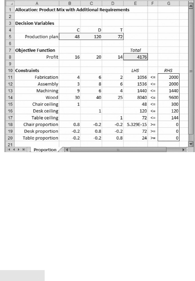
Appending these three constraints to the product mix model gives rise to the linear

program described in Figure 2.16. In the ﬁgure, we show the spreadsheet after the

model has been optimized. Before the constraints were added, the optimal mix gener-

ated proﬁts of $4672. With the 20 percent ﬂoor imposed, we expect optimal proﬁts to

drop. As shown in Figure 2.16, the new optimal mix becomes 48 chairs, 120 desks,

and 72 tables. Thus, swapping chairs for tables in the product mix, we can achieve

the best possible level of proﬁt, achieving a total of $4176. As we might have expected,

chairs make up exactly 20 percent of the optimal output in this solution, while desks

and tables each account for more than 20 percent.

Whenever we encounter a constraint in the form of a lower limit or an upper limit

on a proportion, we can follow similar steps.

Chapter 2 Linear Programming: Allocation, Covering, and Blending Models

†

Write the fraction that expresses the constrained proportion.

†

Write the inequality implied by the lower limit or upper limit.

†

Multiply through by the denominator and collect terms.

The result should be a linear inequality, ready to incorporate in the model.

In general, the blending problem involves mixing materials that have different

individual properties and describing the properties of the blend with weighted

averages. We might be familiar with the phenomenon of mixing from spending

time in a chemistry laboratory mixing ﬂuids with different concentrations of a particu-

lar substance, but the concept extends beyond laboratory work. Consider the example

of Keogh Coffee Roasters.

EXAMPLE 2.4

Keogh Coffee Roasters

Keogh Coffee Roasters blends three types of coffee beans (Brazilian, Colombian, and Peruvian)

into ground coffee that is sold at retail. Each kind of bean has a distinctive aroma and taste, and

the company has a chief taster who can rate the fragrance of the aroma and the strength of the

taste on a scale of 1 to 100. The features of the beans are tabulated below.

Figure 2.16. Modiﬁed product mix model.

2.4. Blending Models 49

Aroma Strength Cost per

Bean Rating Rating Pound

Brazilian 75 15 $0.50

Colombian 60 20 $0.60

Peruvian 85 18 $0.70

Keogh would like to create a blend that has an aroma rating of at least 78 and a strength rating of

at least 16. However, its supplies of the various beans are limited. The available quantities are

1500 lb of Brazilian, 1200 lb of Colombian, and 2000 lb of Peruvian beans, all delivered under a

previously arranged purchase agreement. Keogh wants to make 4000 lb of the blend at the

lowest possible cost. B

For a little background on blending arithmetic, suppose that we blend Brazilian

and Peruvian beans in equal quantities of 25 lb each. Then we should expect the

blend to have an aroma rating of 80, just halfway between the two pure ratings of

75 and 85. Mathematically, we take the weighted average of the two ratings

Aroma rating =

75(25) + 85(25)

25 + 25

4000

= 80

Now suppose that we blend the beans in amounts B, C, and P. The blend has an aroma

rating calculated by a weighted average of the three ratings

Aroma rating =

75B + 60C + 85P

B + C + P

To impose a constraint that requires the aroma rating to be at least 78, we write

75B + 60C + 85P

B + C + P

≥ 78

Once again, this constraint is nonlinear, by virtue of having decision variables in the

denominator of the fraction. However, as shown above, we can convert the require-

ment into a linear constraint. First, multiply both sides of the inequality by (B +

C + P), yielding

75B + 60C + 85P ≥ 78(B + C + P)

Next, collect terms involving the decision variables on the left-hand side, to obtain

−3B − 18C + 7P ≥ 0

This form conveys the same requirement as the original fractional constraint, but in

linear form. The coefﬁcients on the left-hand side turn out to be just the differences

between the individual aroma ratings (75, 60, 85) and the requirement of 78, with

signs indicating whether the individual rating is above or below the target. In a similar

fashion, a requirement that the strength of the blend must be at least 16 leads to the

constraint

−1B + 4C + 2P ≥ 0

Chapter 2 Linear Programming: Allocation, Covering, and Blending Models

In general, the natural way to describe a blending requirement uses fractions, but

in that form, blending requirements are nonlinear. We prefer to convert these require-

ments to linear constraints because with a linear model we can harness the full power

of the linear solver. As we shall see later, the nonlinear solver has more limitations than

the linear solver.

Now, with an idea of how to restate the blending requirements, we return to

Example 2.4. In addition to the blending constraints, we need a constraint that gener-

ates a 4000-lb blend, along with three constraints that limit the supplies of the different

beans. The algebraic problem statement is as follows.

Maximize z = 0.50B + 0.60C + 0.70P

subject to

− 3B − 18C + 7P ≥ 0

− 1B + 4C + 2P ≥ 0

B + C + P ≥ 4000

B ≤ 1500

C ≤ 1200

P ≤ 2000

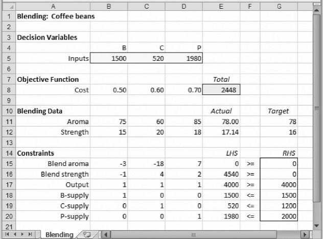
Figure 2.17 shows the spreadsheet for our model, which contains a GT constraint

and three LT constraints, in addition to the two blending constraints. In a sense, the

Figure 2.17. Keogh Coffee Roasters model.

2.4. Blending Models 51

model has what we might think of as covering and allocation constraints, in addition to

blending constraints. The Blending Data module, in rows 10–12, is not strictly part of

the optimization model. We’ll come back to this part of the worksheet later. Each con-

straint in rows 15–20 is expressed in our standard form: a SUMPRODUCT formula

on the LHS and a parameter on the RHS. This model contains three LT constraints and

three GT constraints. It is helpful to keep constraints of the same type in adjacent

locations on the worksheet, for convenience in entering the constraint information

in the task pane. In this case, with only two entries in the Add Constraint window,

we can specify all six inequalities.

The output constraint is formulated as an inequality. Although Keogh Coffee

Roasters wishes to produce 4000 lb, our model allows the production of a larger quan-

tity if this will reduce costs. (Our intuition probably tells us that we should be able to

minimize costs with a 4000-lb blend, but we would accept a solution that reduced costs

while producing more than 4000 lb: we could simply throw away the excess.) In many

situations, it is a good idea to use the weaker form of the constraint, giving the model

some “additional rope” and avoiding EQ constraints. In other words, we should build

the model with some latitude in satisfying the constraints of the decision problem

whenever possible. The solution will either conﬁrm our intuition (as this one does)

or else teach us a lesson about the limitations of our intuition.

The model speciﬁcation is the following

Objective:

Variables:

Constraints:

E8 (minimize)

B5:D5

E15:E17 ≥ G15:G17

E18:E20 ≤ G18:G20

The linear solver produces an optimal blend of 1500 lb of Brazilian, 520 lb of

Colombian and 1980 lb of Peruvian beans, for a total cost of $2448, as shown in

the ﬁgure. By using linear programming, Keogh Coffee Roasters can optimize the

cost of its blend while meeting its taste and aroma requirements. Of the two blending

constraints, only the ﬁrst (aroma) constraint is binding in this solution; the optimal

blend actually has better-than-required strength. The output constraint is also binding

(consistent with our intuitive expectation), as is the limit on Brazilian supply.

In Figure 2.19, we calculate the actual aroma and taste ratings in cells E11:E12,

using the weighted-average ratio formula directly. For example, the calculation in cell

E11 uses the formula

=SUMPRODUCT($B$5:$D$5,B11:D11)/E17. Thus, where-

as the ﬁrst constraint of the model is binding (LHS and RHS of row 15 both equal to

zero), the aroma calculation in the Blending Data module shows that the weighted aver-

age equals the requirement of 78 exactly. Although the second constraint shows that the

strength requirement is not binding, the comparison of LHS (4540) with RHS (zero) is

not as helpful as a means of interpreting the slack in the constraint. However, cell E12

shows that the optimal blend’s strength is 17.14, which we can easily compare to the

requirement of 16.

Blending problems arise whenever weighted averages characterize the properties

of a composite product. In our example, we treated taste and aroma as if they were

Chapter 2 Linear Programming: Allocation, Covering, and Blending Models

numerically objective measures, for the purposes of illustration. However, it is not dif-

ﬁcult to enumerate some applications where the parameters are “harder” numbers and

blending concerns are relevant.

†

Gasoline is a blend, and the octane rating of gasoline is a weighted average of

its constituents. The inputs into a gasoline blend have different octane ratings as

a function of their crude oil source and their previous processing steps. The

classiﬁcation of gasoline blends as regular, premium, or super premium is

usually based on a minimum octane rating in each category. The principle of

weighted average blending applies as well to other ﬂuids, such as the viscosity

of lubricants, the sugar content of fruit juice or the fat content of ice cream.

†

Chemical compounds other than ﬂuids often have such constituents as nickel,

copper, sulfur, potassium, and the like. These constituents may have functional

beneﬁts, or they may be considered impurities. In either event, different com-

pounds have different percentage compositions of these elements, and compo-

sitions blend according to weighted averages when elements are mixed

together. The principle of weighted averages applies to metal in alloys, pollu-

tants in emissions, or active ingredients in medications.

†

Investment portfolios consist of discrete assets, such as stocks and bonds. Each

asset in the portfolio has its own ﬁnancial characteristics, but properties of the

overall portfolio dictate admissible investment strategies. The principle of

weighted averages applies to maturities of bonds, rates of return on stocks,

and riskiness ratings of assets.

2.5. MODELING ERRORS IN LINEAR PROGRAMMING

We have presented our examples as if they were built by knowledgeable analysts, with

each step implemented correctly and all errors avoided. However, someone new to the

experience of building optimization models seldom makes it through all of the steps

without some kind of difﬁculty. Even experts run into problems, especially when

they are working on complex models. It is probably unrealistic to expect that the pro-

cess of building and analyzing a model can be carried out without encountering some

sort of difﬁculty along the way. To be effective in modeling, we have to know how to

deal with errors when they occur.

2.5.1. Exceptions

Given a linear programming model, Solver always ﬁnds an optimal solution, provided

one exists. The ﬁrst kind of modeling error is formulating a model that does not have

an optimal solution. Two exceptions can cause difﬁculties: infeasible constraints and

an unbounded objective function.

A model contains infeasible constraints if no set of decision variables can

satisfy all constraints simultaneously. For example, in the product mix example of

2.5. Modeling Errors in Linear Programming 53

Figure 2.9, suppose we had signed a contract promising that 200 chairs would be deliv-

ered to a single large customer, as part of the product mix. Adding the requirement

C ≥ 200 to the other constraints of the model creates an inconsistency. (The implied

machining requirement would be 1800 hours, which exceeds the capacity available.)

Presented with a set of inconsistent constraints, Solver detects the inconsistency and

delivers the following result message in the solution log as well as at the bottom of

the task pane:

Solver could not find a feasible

solution.

Whenever this message appears, there must have been an inconsistency in the set of

constraints.

For the model builder, the task is to locate the inconsistency when confronted with

the infeasibility message. There are potentially two levels to this task: (1) ﬁnding the

offending constraint or constraints, and (2) identifying the source of the inconsistency.

Sometimes, the offending constraint can be discovered by “eyeballing” the model—

scanning for visual clues to the location of an error. For example, a parameter could

be entered incorrectly. (Perhaps the chair contract calls for only 20 units, but 200

has been entered inadvertently.) Alternatively, a constraint could be entered backward,

as a LT constraint when it should have been a GT constraint. However, the more stan-

dard way to search for an inconsistency is to remove constraints from the model, one

at a time, and to rerun Solver each time. (In large problems, it might make more sense

to remove several constraints at a time.) If the model remains infeasible, restore the

constraint and try removing a different one. If the model reaches an optimal solution,

then we know that something about the constraint we removed was a partial cause of

the infeasibility.

Identifying the source of an inconsistency refers to the part of the task that lies at

the interface between model and problem. If the inconsistency resulted from a ty po,

then it is a simple matter to repair it. However, a more subtle difﬁculty arises when

the formulation contains too many constraints. This result can occur if, during the

modeling process, there was a thorough attempt to include all the considerations men-

tioned by various parties. Isolated desires and secondary considerations could wind up

being expressed as model constraints, contributing to a logical conﬂict. In th ese situ-

ations, it makes sense to eliminate some of the constraints, so that the model is at least

feasible. Thereafter, various additional considerations can be revisited, to see whether

they can be accommodated without causing infeasibility.

The second kind of modeling error occurs when there is no limit to the objective

function in the direction of optimization. An unbounded objective function occurs if,

with a set of feasible decisions, the objective can grow inﬁnitely positive in a maximi-

zation problem or inﬁnitely negative in a minimization problem. The most common

cause of an unbounded objective is failure to invoke the Assume Non-Negative

option. For example, in the trail mix example of Figure 2.11, suppose we had forgotten

to set the option to True. Then it would be mathematically possible to make the objec-

tive function as negative as we wish by taking negative quantities for some of the

ingredients. Consider the mix corresponding to R ¼ 115, P ¼ –40, and W ¼ –50.

Chapter 2 Linear Programming: Allocation, Covering, and Blending Models

This combination satisﬁes all four constraints, with a total cost of – $5.00. Mathemat-

ically, this mix could be expanded in the same proportion, with all constraints met

and the total cost becoming as negative as we like. Presented with conditions that

permit an objective function to expand inﬁnitely in the direction of optimization,

Solver detects the unbounded possibilities and delivers the following result message

in the solution log as well as at the bottom of the task pane:

The objective (Set Cell) values do

not converge.

The reference to “Set Cell” provides consistency with older versions of the software,

which did not use the term “objective.”

For the model builder, the task is to locate the cause of an unbounded objective

function. The problem could lie in the objective function or in the constraints. A

simple typo in an objective function cell could induce unbounded possibilities.

However, unboundedness can also occur when a constraint is omitted from the

model, allowing decision variables to reach values never intended by the model

builder. Whereas locating the cause of infeasibility directs attention to the constraints,

it is more difﬁcult to know where to look for the cause of unboundedness.

2.5.2. Debugging

Even a model that contains feasible constraints and a bounded objective function can

be logically ﬂawed. Beyond its ability to detect infeasible and unbounded formu-

lations, Solver has no automatic means of detecting logical errors. That responsibility

lies with the model builder. However, a few techniques that are helpful to spreadsheet

users can augment the capabilities in Solver.

†

Set all decision variables to zero. A good ﬁrst step is to enter zero for each of

the decision variables and conﬁrm that the objective function and constraints

behave as expected. Then, make one variable at a time positive. Taking succes-

sive values for a variable equal to 1, 10, and 100 can show whether the scaling

properties of the model seem valid.

†

Display formulas. By simultaneously pressing the Control and tilde ()keys,

we can look at all the formulas in the spreadsheet window. As in Figure 2.2, we

look for the SUMPRODUCT formulas in the cells corresponding to the objec-

tive function and the LHS of each constraint. No other formulas are necessary,

although in the next chapter we shall look at some cases where an alternative

form is convenient. Pressing the Control and tilde keys simultaneously once

more restores the display.

†

Invoke Formula Auditing. The Formula Auditing tools appear on the Formulas

tab. In Figure 2.18, we have selected, one at a time, each of the constraint for-

mulas and selected the Trace Precedents icon for each one. The resulting logical

map exhibits a systematic structure that helps validate the formulas. An

2.5. Modeling Errors in Linear Programming 55