Baker K.R. Optimization Modeling with Spreadsheets

Подождите немного. Документ загружается.

usually of two types: capacity constraints on production resources and demand con-

straints on potential sales. In Example 2.1, suppose that the company markets its

chairs, tables, and desks through a distributor who also provides monthly forecasts

of demands. Next month’s forecasts are:

Chairs Desks Tables

Demand 300 120 144

With this information, we can extend the basic allocation model to include three

demand constraints as well. The full model takes the following algebraic form.

Maximize z = 16C + 20D + 14T

subject to

4C + 6D + 2T ≤ 2000

3C + 8D + 6T ≤ 2000

9C + 6D + 4T ≤ 1440

30C + 40D + 25T ≤ 9600

C ≤ 300

D ≤ 120

T ≤ 144

The spreadsheet version of this model simply adds three rows to the model in

Figure 2.6. Most easily, the LHS formula can be copied from the wood supply con-

straint (cell E14) into cells E15:E17 after the new coefﬁcients have been added, as

shown in Figure 2.7.

We must then update the model speciﬁcation so that all seven constraints are

included. To make this adjustment most simply, we can select the range E15:E17

and add the corresponding constraints via the Add Constraint window. The updated

representation in the window of the Model tab lists two sets of constraints, as

shown in Figure 2.8. Although it may not be necessary in every case, it is a good

habit to click the Refresh icon after adding or deleting variables or constraints, so

we do that here.

Alternatively, to update the allocation model, we can double-click on the icon for

the existing Normal constraints, which opens the Change Constraint window. This

time, we can edit the Cell Reference box and the Constraint box so that the ranges

include all seven of the constraints. Then, the window on the Model tab displays

only one set of constraints. Again, it is a good habit to click Refresh.

A new optimization run then reveals that the optimal product mix becomes 16

chairs, 120 desks, and 144 tables, as shown in Figure 2.9. The optimal proﬁt contri-

bution in the product mix model is $4672. This amount is less than the optimal

proﬁt in the original allocation model. Not surprisingly, the imposition of demand ceil-

ings leads to a reduction in the optimal proﬁt. In fact, looking back at Figure 2.7, we

Chapter 2 Linear Programming: Allocation, Covering, and Blending Models

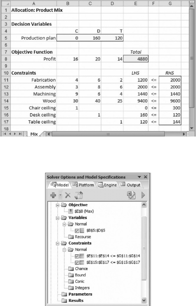
Figure 2.8. Specifying additional constraints.

Figure 2.7. Product mix model.

2.2. Allocation Models 37

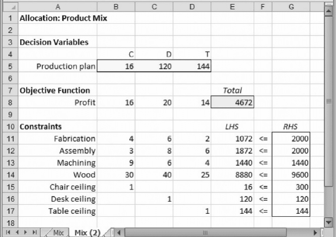
can see immediately that the product mix of 160 desks and 120 tables does not meet all

of the demand ceiling constraints. This outcome illustrates the intuitive principle that

the addition of constraints to a model cannot improve the optimal objective function—

it will be the same or worse when constraints are added.

Three binding constraints occur in the product mix model: the demand ceiling

for desks, the demand ceiling for tables, and machining capacity. None of the other

constraints is binding.

In general, the product mix model involves different types of capacity and perhaps

different types of demand. For example, in our scenario, the different types of capacity

are labor, equipment, and material inputs for production. Alternatively, the labor might

be broken down into regular-time and overtime hours, or the material could come from

“make” versus “buy” sources (i.e., from in-house fabrication and assembly or from an

outside subcontractor). Similarly, demand could be speciﬁed by geographical region

or by time period, the latter for a multiperiod formulation. In the multiperiod case, it is

usually helpful to keep track of inventory levels, partly because inventories affect costs

but also because inventory can be considered yet another source of product, just like

regular-time capacity or subcontracted production. One common variation of the basic

product mix model is to include GT constraints on potential sales of certain products.

A minimum demand quantity might reﬂect a contractual commitm ent or represent a

sales level that management wishes to meet under any circumstances. Such demand

thresholds may or may not be part of the model; the distinctive features of the product

Figure 2.9. Optimal Solution to the product mix model.

38 Chapter 2 Linear Programming: Allocation, Covering, and Blending Models

mix model are capacity constraints on productive resources and demand constraints on

market requirements.

2.3. COVERING MODELS

The covering problem calls for minimizing an objective (usually cost related) subject

to GT constraints on required coverage. Whereas the allocation model divides

resources and assigns them to competing activities, the covering model combines

resources and coordinates activities. Consider the example of Herrick Foods

Company.

EXAMPLE 2.2

Herrick Foods Company

Herrick Foods Company wishes to introduce packaged trail mix as a new product. The ingredi-

ents for the trail mix are seeds, raisins, ﬂakes, and two kinds of nuts. Each ingredient contains a

certain amount of vitamins, minerals, protein, and calories; and the Marketing Department has

speciﬁed the product be designed so that a certain minimum nutritional proﬁle is met. The

decision problem is to minimize the product cost and determine the product composition—

that is, by choosing the amount of each ingredient in the mix. The data shown below summarize

the parameters of the problem.

Grams per pound

Nutritional

Seeds Raisins Flakes Pecans Walnuts requirement

Vitamins 10 20 10 30 20 16

Minerals 5 7 4 9 2 10

Protein 1 4 10 2 1 15

Calories 500 450 160 300 500 600

Cost/pound $4 $5 $3 $7 $6

To determine the decision variables, we again ask, “What must be decided?” The

answer is we need to determine the amount of each ingredient to put in a package of

trail mix. For the purposes of notation, we can use S, R, F, P, and W to represent the

number of pounds of each ingredient in a package.

Next, we ask, “What measure will we use to compare sets of decision variables?”

This should be the total cost of a package, and our interest lies in the lowest possible

total cost. To calculate the total cost of a particular composition, we sum the costs of

each ingredient in the package

Cost = 4S + 5R + 3F + 7P + 6W

To identify the model’s constraints, we ask, “What restrictions limit our choice of

decision variables?” In this scenario, the main limitation is the requirement to meet the

2.3. Covering Models 39

speciﬁed nutritional proﬁle. Each dimension of this proﬁle gives rise to a separate con-

straint. An example of such a constraint states, in words, that the number of grams of

vitamins provided in the package must be greater than or equal to the number of grams

required by the speciﬁed proﬁle. Laying out those words in the format of an inequality,

we can write

Grams of vitamins provided ≥ Grams of vitamins required

where we chose to place “grams required” on the RHS because it is represented by a

parameter of the model (16 grams, in this case). Converting the inequality to symbols,

we can then write

Vitamin content = 10S + 20R + 10F + 30P + 20W ≥ 16 (Vitamin floor)

Similar constraints must hold for mineral protein, and calorie content. The entire

model, stated in algebraic terms, reads as follows.

Minimize z = 4S + 5R + 3F + 7P + 6W

subject to

10S + 20R + 10F + 30P + 20W ≥ 16

5S + 7R + 4F + 9P + 2W ≥ 10

1S + 4R + 10F + 2P + 1W ≥ 15

500S

+ 450R + 160F + 300P + 500W ≥ 600

In this basic scenario, no other constraints arise, although we could imagine that there

could also be limited quantities of the ingredients available, expressed as LT con-

straints, or a weight requirement for the package, expressed as an EQ constraint.

A spreadsheet model for the basic scenario appears in Figure 2.10. Again, we see

the three modules: a highlighted row for decision variables, a highlighted single cell

for the objective function value, and a set of constraint relationships with highlighted

RHS’s. If we were to displ ay the formulas for this model, we would again see that the

only formula in the worksheet is the SUMPRODUCT formula.

Once we have persuaded ourselves that the model is valid, we proceed to the

Model tab in the task pane and enter the following information

Objective:

Variables:

Constraints:

G8 (minimize)

B5:F5

G11:G14 ≥ I11:I14

As in the allocation model, we move to the Engine tab, specify the linear solver, and

invoke the option for nonnegative variables.

After contemplating some hypotheses about the problem (e.g., will the solution

require all ﬁve ingredients?) we run Solver and ﬁnd the result message in the solution

log. The optim al solution is reproduced in Figure 2.11. It calls for 0.48 lb of seeds,

0.33 lb of raisins, and 1.32 lb of ﬂakes, with no nuts at all. Evidently, nuts are prohi-

bitively expensive, given the nature of the required nutritional proﬁle and the other

Chapter 2 Linear Programming: Allocation, Covering, and Blending Models

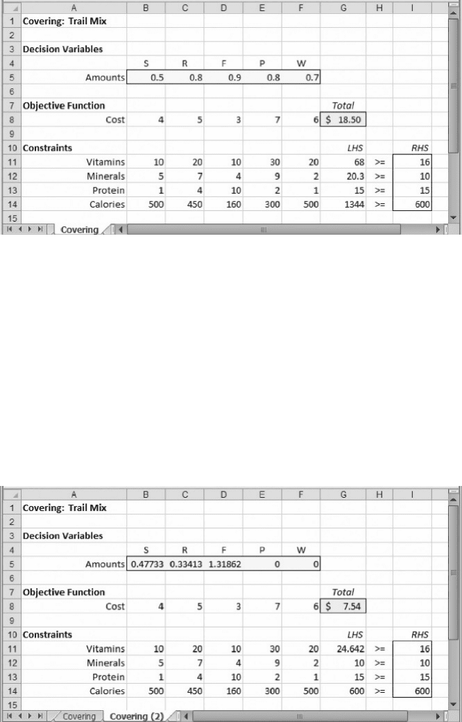
ingredients available. The optimal mix achieves all of the nutritional requirements at a

minimum cost of $7.54. The tight constraints in this solution are the requirements for

minerals, protein, and calories.

Herrick Foods might decide that trail mix without nuts is not an appealing pro-

duct. This concern illustrates another situation where the solution to the model may

not represent a solution to the practical problem. In building the model, we have not

considered the implication of a product without nuts. Alerted to this possibility, we

may wish to revisit the model and make sure that some nuts appear in the optimal

mix. One way to do so is to require a minimum of 0.15 lb of both pecans and walnuts

Figure 2.11. Optimal solution for the Herrick Foods model.

Figure 2.10. Model for Herrick Foods example.

2.3. Covering Models 41

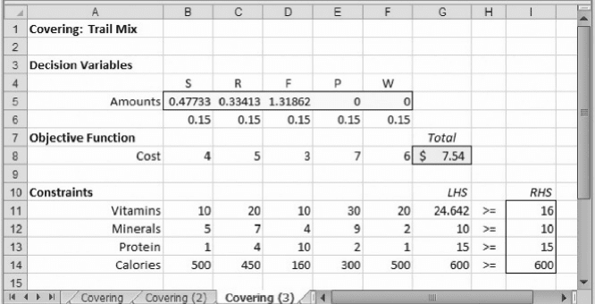
in the mix. In Figure 2.12, we show an amended model that requires at least 0.15 lb of

every ingredient.

The value of 0.15 appears just below the corresponding decision variable, and in

the Model tab of the task pane, we add the constraint that the range B5:F5 must be

greater than or equal to the range B6:F6. After this update, we revise the model

speciﬁcation as follows

Objective:

Variables:

Constraints:

G8 (minimize)

B5:F5

B5:F5 ≥ B6:F6

G11:G14 ≥ I11:I14

The requirement that a particular decision variable must be greater than or equal to a

given value is called a lower bound constraint. Here, the ﬁrst set of constraints is for-

mulated as a range of lower bound constraints. Similarly, a requirement that a particu-

lar decision variable must be less than or equal to a given value would be called an

upper bound constraint. (We could have used such constraints in the product mix

model, but in Figure 2.9 we posed them in the standard SUMPRODUCT style, so

that they resembled the other constraints in the model.)

After including the lower bound constraints, running Solver again produces the

optimal solution shown in Figure 2.13. By using linear programming and acknowled-

ging a requirement to include all ﬁve ingredients in the ultimate mixture, Herrick

Foods has identiﬁed the desired composition of its trail mix product.

Imposing lower bounds on the original Herrick Foods model leads to an optimal

solution that contains all ﬁve of the ingredients. We might have expected that nuts

would appear exactly at their lower limit because without the lower boun d constraints,

the optimization left nuts completely out of the solution. Thus, when we added the

lower bound, there was no incentive to include nuts at any level greater than the

Figure 2.12. Herrick Foods model with additional constraints.

42 Chapter 2 Linear Programming: Allocation, Covering, and Blending Models

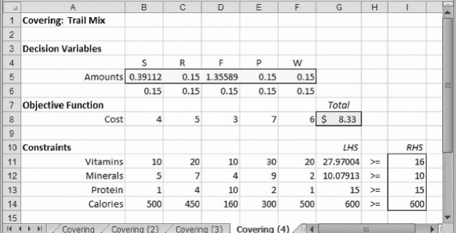
lower bound. The optimal cost is also higher in the amended model than in the orig-

inal, at $8.33. This result again reﬂects the intuitive principle that adding constraints to

a model cannot improve the objective function—it will be the same or worse when

constraints are added.

The trail mix example is a simpliﬁed version of a classic covering problem known

as the diet problem. This problem arises, for example, in the determination of weekly

menus for large institutional populations, such as those in nursing homes, prisons, and

summer camps. The purpose of the model is to determine meal selection for each of

the 21 meals served each week to everyone in a large group. The variables may rep-

resent quantities of various food groups (meats, vegetables, fruits, etc.), and weekly

nutritional requirements reﬂect limits on the totals of weekly requirements for fat, cal-

ories, protein, carbohydrates, and so on. A common phenomenon, akin to the results of

our ﬁrst trail mix model, is that cost minimization drives the solution toward a limited

number of meals. Camp ers may not ﬁnd a steady diet of tofu appealing, even if that is

the model’s optimal solution. Subtle differences between the problem and the model

become clearer once a solution is obtained. For that reason, a more detailed and com-

plicated set of constraints must often be added to the diet model in order to generate an

appetizing weekly menu.

2.3.1. The Staff-Scheduling Problem

Many service industries face the problem of scheduling their workforce to meet ﬂuc-

tuating stafﬁng requirements. Nurses, telephone operators, toll collectors, and bus dri-

vers operate in this type of environment—providing service over a period that extends

beyond the normal 8 hr working day and possibly continuing around the clock. Many

companies restrict themselves to full-time workers and they meet ﬂuctuating

Figure 2.13. Optimal solution to the modiﬁed Herrick Foods model.

2.3. Covering Models 43

requirements of this sort by assigning staff to overlapping work shifts. As an example,

consider the daily stafﬁng problem at Acme Communications.

EXAMPLE 2.3

Acme Communications

Acme Communications operates a regional call center where the workday is broken down into

six 4-hour shifts, and each operator works two consecutive shifts. The table below describes staff

requirements on each shift.

Shift number #1 #2 #3 #4 #5 #6

Time period 2 am–6 am 6 am– 10 am 10 am–2 pm 2 pm–6 pm 6 pm–10 pm 10 pm– 2 am

Requirement 10 20 45 40 50 12

The call center’s manager wishes to assign operators to the six available starting times so that

the stafﬁng requirements are covered in each period and the total workforce size is as small

as possible. B

For Acme’s problem, the decision variables are the number of operators assigned

to each of the six starting times. For example, let x

represent the number assigned to

begin work on shift #1. These operators work during shifts #1 and #2, from 2 am to

10 am. Similarly, x

represents the number assigned to work during shifts #2 and

#3, from 6 am to 2 pm. With this notation, the number of operators working during

shift #2 must equal x

+ x

. By a similar logic, the number of operators working

during shift #3 must equal x

+ x

, and so on. Finally, the number working during

shift #1 must equal x

+ x

because the requirements repeat in 24-hour cycles. An

algebraic statement of the problem is shown below.

Minimize z = x

+ x

subject to

+ x

≥ 10

+ x

≥ 20

+ x

≥ 45

+ x

≥ 40

+ x

≥ 50

+ x

≥ 12

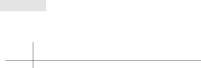
Figure 2.14 shows a spreadsheet model for this problem.

Stafﬁng models of this sort have a distinctive structure. First, because the number

of operators working on any given shift is the total assigned to two starting times, two

variables appear in each constraint. Thus, in the spreadsheet, there are two 1s on the

LHS of each constraint row. Second, because operators work two consecutive

Chapter 2 Linear Programming: Allocation, Covering, and Blending Models

shifts, two consecutive 1s appear in the columns corresponding to variables. (In the

case of x

, shifts #6 and #1 are consecutive.) The model speciﬁcation is as follows

Objective:

Variables:

Constraints:

H8 (minimize)

B5:G5

H11:H16 ≥ J11:J16

Figure 2.14 displays an optimal solution, which achieves a total workforce of 105 by

assigning various numbers of operators to ﬁve starting times, with no one starting

work at 10 pm.

In general, we can structure the staff-scheduling model around the shift deﬁnition.

Time periods correspond to rows in the model and alternative shift assignments cor-

respond to columns. For a problem in which the assignments correspond to days, we

can imagine seven constraint s (each one representing a daily stafﬁng requirement) and

seven assignments (each one corresponding to a different start of a 5-day work stretch).

In the constraints module, the column of coefﬁcients under a given shift assignment

shows the proﬁle of the work shift. In Figure 2.14, those coefﬁcients are two consecu-

tive 1s, reﬂecting the fact that each assignment comprises two consecutive 4-hour time

periods. In a more detailed version with 2-hour time periods, we can imagine four con-

secutive 1s. In an hourly version, we can imagine eight consecutive 1s. In most appli-

cations, however, when the time periods are this detailed, provisions are usually made

for meal breaks as well. As an example, imagi ne a service facility that operates over a

12-hour span from 6 am to 6 pm. Shifts begin on the hour and contain 8 hours of work

Figure 2.14. Stafﬁng model.

2.3. Covering Models 45