Baker K.R. Optimization Modeling with Spreadsheets
Подождите немного. Документ загружается.

deploy, quantities to produce, or quantities to deliver. Whatever the decision variables
are, once we know their numerical values, we should have a resolution to the problem,
though not necessarily the best resolution.
To guide us toward an objective function, we ask ourselves, “What measure will
we use to compare sets of decision variables?” It is as if two consultants have come to
us with their recommendations on what action to take (what levels of the decision vari-
ables to use), and we must choose which action we prefer. For this purpose, we need a
yardstick—some measuring function that tells us which action is better. That function
will be a mathematical expression involving the decision variables, and it will nor-
mally be obvious whether we wish to maximize or minimize it. Maximization criteria
usually focus on such measures as profit, revenue, return, or efficienc y. Minimization
criteria usually focus on cost, time, distance, capacity, or investment. In the model,
only one measure can play the role of the objective function.
To guide us toward constraints, we ask ourselves, “What restrictions limit our
choice of decision variables?” We are typically not free to choose any set of decisions
we like; intrinsic limitations in the problem have to be respected. For example, we
might look for capacities that provide upper limits on certain activities and give rise
to LT constraints. Alternatively, there may be commitments that place thresholds on
other activities, in the form of GT constraints. Sometimes, we wish to specify
equations, or EQ constraints, that ensure consistency among a set of variables.
Once we have identified the constraints in a problem, we say that any set of decision
variables consistent with all the constraints is a feasible solution. That is, a feasible
solution represents a course of action that does not violate any of the constraints.
Among feasible solutions, we want to find the best one.
It is usually a good idea to identify decision variables, objective function, and
constraints in words first, and then translate them into algebraic symbols. The alge-
braic step is useful when we practice the formulation of optimization models
because it helps us to be precise at an early modeling stage. In addition, an algebraic
formulation can usually be translated into a spreadsheet model directly, although we
may wish to make adjustments for the spreadsheet environment. As indicated in
Chapter 1, it is desirable to create as much transparency as possible in the spreadsheet
version of a model, therefore, our approach will be to construct an algebraic formula-
tion as a prelude to creating the spreadsheet model.
2.1.3. Layout
We follow a disciplined approach to building linear programming models on a spread-
sheet by imposing some standardization on spreadsheet layout. The developers
of Solver provided model builders with considerable flexibility in designing a spread-
sheet for optimization. However, even those developers recognized the virtues of some
standardization, and their user’s manual conveys a sense that taking full advantage
of the software’s flexibility is not always consistent with best practice. We adopt
many of their suggestions about spreadsheet design.
26
Chapter 2 Linear Programming: Allocation, Covering, and Blending Models
The first element of our structure is modularity. We should try to reserve separate
portions of the worksheet for decision variables, objective function, and constraints.
We may also want to devote an additional module to raw data, especially in large pro-
blems. In our basic models, we should try to place all decision variables in adjacent
cells of the spreadsheet (with color or border highlighting). Most often, we can display
the variables in a single row, although in some cases the use of a rectangular array is
more convenient. The objective function should be a single cell (also highlighted),
containing a SUMPRODUCT formula, although in some cases an alternative may
be preferable. Finally, we should arrange our constraints so that we can visually com-
pare the LHS’s and RHS’s of each constraint, relying on a SUMPRODUCT formula
to express the LHS, or in some cases, a SUM formula. For the most part, our models
can literally reflect left and right in the layout, although sometimes other forms also
make sense.
The rel iance on the SUMPRODUCT function is a conscious design strategy. As
mentioned earlier, the SUMPRODUCT function is intimately related to linearity. By
using this function, we can see structural similarities in many apparently different
linear programs, and the recognition of this similarity is key to our understanding.
Moreover, by taking this approach, we can build recognizable models in a standard
format for virtually any linear programming problem (although other approaches
may be better for certain circumstances). In addition, the SUMPRODUCT function
has technical significance. Solver is designed to exploit the use of this function,
mainly in setting up the problem quickly for internal calculations. This becomes an
advantage in large models, so it makes sense to learn the habit while practicing on
smaller models.
With the partial standardization implied by these “best practice” guidelines, we
may be restricting the creative instinct somewhat, but we gain in several important
respects.
†
We enhance our ability to communicate with others. A standardized structure
provides a common language for describing linear programs and reinforces
our understanding about how such models are shaped. This is especially true
when spreadsheet models are being shown to technical experts.
†
We improve our ability to diagnose errors while building the model. A standar-
dized structure has certain recognizable features that help us detect modeling
errors or simple typos. In a spreadsheet context, we often exploit the ability
to copy a small number of cell formulas to several other locations, so we can
avoid some common errors by entering part of the standard structure carefully
and then copying it appropriately.
†
We make it relatively easy to “scale up” the model. That is, we may want to
expand a model by adding variables or constraints, allowing us to move
from a prototype to a practical scale or from a “toy” problem to an “industrial
strength” version. The standard structure adapts readily when we wish to
expand a model this way.
2.1. Linear Models 27
†
We avoid some interpretation problems when we perform sensitivity analysis.
A standardized structure ensures that Solver will treat the spreadsheet infor-
mation in a dependable fashion. Otherwise, sensitivity analyses may become
ambiguous or confusing.
2.1.4. Results
Just as there are three important modules in our spreadsheet (decision variables, objec-
tive function, and constraints), there are three kinds of information to examine in the
optimization results.
†
The optimal values of the decision variables indicate the best course of action
for the model.
†
The optimal value of the objective function specifies the best level of perform-
ance in the model.
†
The status of the constraints reveals which factors in the model truly prevent the
achievement of even better levels of performance.
In particular, a LT or GT constraint in which the LHS equals the RHS is called
a tight or a binding constraint. Prior to solving the model, each constraint is a potential
limitation on the set of decisions, but the optimization of the model identifies which
constraints are actual limitations. These are the physical, economic, or administrative
conditions in the problem that actively restrict the ultimate performance level.
We can think of the solution to a linear program as providing what we might call
both tactical and strategic information. Tactical information means that the optimal
solution prescribes the best possible set of decisions under the given conditions.
Thus, if the model represents an actual situation, its optimal decisions represent a
plan to implement. Strategic information means that the optimal solution identifies
which conditions prevent the achievement of bett er levels of performance. In particu-
lar, the model’s binding constraints indicate the factors that restrict the objective func-
tion. If we don’t have to implement a course of action immediately, we can explore the
possibility of altering one or more of those constraints in a way that improves the
objective. Thus, if the model represents a situation with given parametric conditions,
and we want to improve the level of performance, we can examine the possibility of
changing the “givens.”
Whether we have tactical information or strategic information in mind, we must
still recognize that the optimization process finds a solution to the model, not necess-
arily to the actual problem. The distinction between model and problem derives
from the fact that the model is, by its very nature, a simplification. Any features of
the problem that were assumed away or ignored must be addressed once we have a
solution to the model. For example, a major assumption in linear programs is that
all of the model’s parameters are known with certainty. Frequently, however, we
find that we have to work with uncertain estimates of model parameters. In that situ-
ation, it is important to examine the sensitivity of the model’s results to alternative
assumptions about the values of the parameters.
28
Chapter 2 Linear Programming: Allocation, Covering, and Blending Models

2.2. ALLOCATION MODELS
We now proceed with our tour of the basic linear programming types. The allocation
problem calls for maximizing an objective (usually profit-related) subject to LT con-
straints on capacity. In the traditional economic paradigm, several activities compete
for limited resources, and we seek the best allocation of resources among the compet-
ing activities. Consider the example of Brown Furniture Company.
EXAMPLE 2.1
Brown Furniture Company
Brown Furniture Company makes three kinds of office furniture: chairs, desks, and tables. Each
product requires skilled labor in the parts fabrication department, unskilled labor in the assembly
department, machining on some key pieces of equipment, and some wood as raw material. At
current prices, the unit profit contribution for each product is known, and the company can sell
everything that it manufactures. The size of the workforce has been established, so the number
of skilled and unskilled labor hours are known. The time available on the relevant equipment
has also been determined, and a known quantity of wood can be obtained each month under
a contract with a wood supplier. Managers at Brown Furniture would like to maximize their
profit contribution for the month by choosing production quantities for the chairs, desks, and
tables. The data shown below summarize the parameters of the problem.
Requirements per unit
Chairs Desks Tables Resources available
Fabrication (hr) 4 6 2 2000 hr
Assembly (hr) 3 8 6 2000 hr
Machining (hr) 9 6 4 1440 hr
Wood (sq. ft) 30 40 25 9600 sq. ft
Profit per unit $16 $20 $14
B
The data in Example 2.1 would likely come from several sources. The number of
labor hours available might be a parameter supplied by the Human Resources
Department. The labor required for each product more likely comes from the
Production Department, and the contract quantity for wood might come from
Procurement. Unit profit contributions can be calculated from information on selling
prices and unit costs, which could come from the Marketing and Accounting
Departments. In short, the kind of data needed for optimization analysis can often
be found in various parts of an organization, and the process of data gathering requires
communication with several functions of the firm. Although we won’t discuss the
details of data sources for most of the other examples in this book, the point is a general
one. Data needed for optimization are seldom found in just one place. More typically,
we have to pursue an interfunctional network of contacts to obtain the data we need for
modeling.
2.2. Allocation Models 29
To build a model for this problem, we follow the outline of Box 2.3. To determine
decision variables, we ask, “What must be decided?” The answer is the product mix, so
we define decision variables as the numbers of chairs, desks, and tables. For the pur-
poses of notation, we can use C, D, and T to represent the number of chairs, the number
of desks and the number of tables, respectively.
Next, we ask, “What measure will we use to compare sets of decision variables?”
If two people in the organization were to advocate two different production plans, we
would respond by calculating the total profit contribution for each one and choosing
the larger value. To calculate profit contribution, we add the profit from chairs, the
profit from desks, and the profit from tables. Thus, an algebraic expression for total
profit becomes:
Profit = 16C + 20D + 14T
To identify the model’s constraints, we ask, “What restrictions limit our choice of
decision variables?” This scenario describes four resource capacities. In words, a pro-
duction capacity constraint might state that the resources consumed in a production
plan must be less than or equal to the resources available. Laying out those words
in the form of an inequality, we can write:
Fabrication hours consum ed ≤ Fabrication hours available
where we chose to place “hours available” on the RHS because it is represented by
a parameter of the model (2000 hours, in this case). Converting the inequality to
symbols, we can then write:
Fabrication hours consumed = 4C + 6D + 2T
≤ 2000 (Fabrication hours available)
Similar constraints must hold for the assembly hours, machining time, and wood
supply:
Assembly hours consumed = 3C + 8D + 6T ≤ 2000 (Assembly hours available)
Machining time consumed = 9C + 6D + 4T ≤ 1440 (Machining time available)
Wood consumed = 30C + 40D + 25T ≤ 9600 (Wood available)
We now have four constraints that describe the restrictions limiting our choice of
decision variables C, D, and T. The entire model, stated in algebraic terms, reads as
follows:
Maximize z =
16C + 20D + 14T
subject to
4C + 6D + 2T ≤ 2000
3C + 8D + 6T ≤ 2000
9C + 6D + 4T ≤ 1440
30C + 40D + 25T ≤ 9600
30
Chapter 2 Linear Programming: Allocation, Covering, and Blending Models
This algebraic statement reflects a standard format for linear programs. Each variable
corresponds to a column and each constraint corresponds to a row, with the objective
function appearing as a special row at the top of the model. This layout is suitable for
spreadsheet display as well.
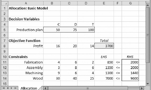
A spreadsheet model for the allocation problem appears in Figure 2.1. Three
modules appear in the spreadsheet, including a highlighted row for the decision vari-
ables, a highlighted s ingle cell for the objective function value, and a set of constraint
relationships in which the RHS values are highlighted. The cells containing the
symbol ,¼ have no function in the operation of the spreadsheet; they are intended
as a visual aid to the user, helping to convey the information in the constraints. We
place them between the LHS value of the constraint (a formula) and the RHS value
(a parameter).
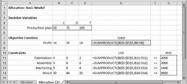
Figure 2.2 shows the formulas in this model. Aside from labels, the model con-
sists of only two kinds of cells: those containing numbers and those containing a
SUMPRODUCT formula. This is our standard form for a linear program in a
spreadsheet.
Figure 2.1 contains an arbitrary set of values for the decision variables (50 chairs,
75 desks, and 100 tables). We could try different sets of three values in order to see
whether we could come up with a good allocation by trial and error. Such an attempt
might also be a useful debugging step, to reassure ourselves that the model is
complete. For example, suppose we start by fixing the number of desks and tables
at zero and varying the number of chairs. For Fabrication capacity, chairs consume
4 hours each and 2000 hours are available; so we could put 2000/4 ¼ 500 chairs
into the plan (i.e., into cell B5), and the result would be feasible for the first constraint.
However, we can see immediately—by comparing the LHS and RHS values—that
this number requires more machining time than we have available. Therefore, we
Figure 2.1. Model for the Brown Furniture example.
2.2. Allocation Models 31
can reduce the number of chairs to 160 ( just enough to consume all of the machining
hours) and verify that sufficient quantities of the other resources are available to sup-
port this volume. Thus, we obtain a feasible plan and a profit contribution of $2560. If
we rely on desks alone, instead of tables, we run into limits imposed by both machin-
ing capacity and wood supply, resulting in profits of $4800. If we rely solely on tables,
we run into limits imposed by assembly capacity, leading to profits of $4666. Next, we
might try some plans containing two of the three products, or perhaps all three. Such
experiments help us to confirm that the model is working properly and give us a feel
for the profit figures that might be achievable.
After verifying the model in this fashion, we proceed to the optimization pro-
cedure on the Risk Solver Platform tab, clicking the Model icon on the ribbon to
make the task pane visible. We then take the following steps.
†
Select cells B5:D5, then choose Add Variables from the drop-down menu on
the Add icon.
†
Select cell E8, then choos e Add Objective from the drop-down menu on the
Add icon.
†
Select cells E11:E14, then choose Add Constraint from the drop-down menu
on the Add icon.
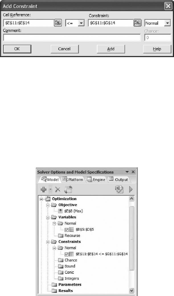
†
Fill in the Add Constraint window requiring that the range E11:E14 must be
less than or equal to G11:G14 (see Figure 2.3). Then press OK.
At this stage the window on the Model tab displays the full specification, as shown in
Figure 2.4.
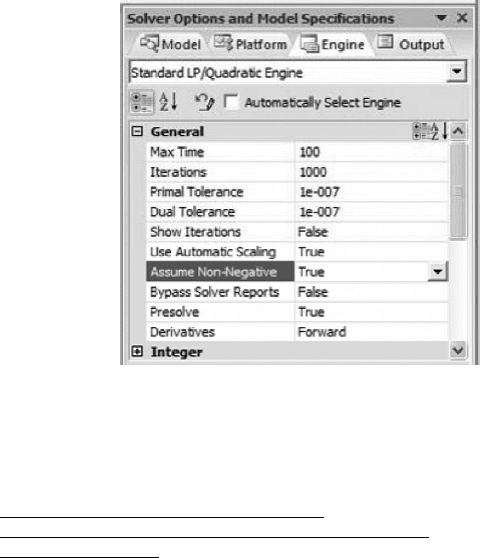
Next, we go to the Engine tab (see Figure 2.5) and take two steps.
†
Select the Standard LP/Quadratic Engine from the drop-down menu. This step
specifies the use of the linear solver.
†
In the main window, set the option for Assume Non-Negative to True.
Figure 2.2. Formulas in the Brown Furniture model.
32 Chapter 2 Linear Programming: Allocation, Covering, and Blending Models
The first of these steps specifies the use of the linear solver. The second makes it
unnecessary to add explicit constraints forcing the variables to be greater than or
equal to zero.
We are now ready for the optimization run, which we can invoke by clicking on
the green triangle icon on either the Model tab or the Output tab. First, however, we
might want to think about some hypotheses. For example, do we expect that the opti-
mal solution will call for all three products? Will it consume all of the available hours?
What order of magnitude should we expect for the optimal profit? This step helps us
build a better intuition for the problem or perhaps discover an error.
Figure 2.4. Specification for the Brown Furniture model.
Figure 2.3. Specifying the constraints.
2.2. Allocation Models 33
If no technical problems occur after we initiate the optimization run, Solver
produces the following result message in the solution log on the Output tab:
Solver found a solution. All
constraints and optimality conditions
are satisfied.
We recognize this as the optimality message, which we encountered in Chapter 1. At
this point the optimal solution is displayed on the spreadsheet.
The linear solver implements a version of the algorithm known as the simplex
method. Although it is not necessary to be acquainted with the simplex method in
order to apply linear programming or to appreciate its significance, some exposure
to the algorit hm may be useful. Appendix 3 provides an algebraic description of the
simplex method.
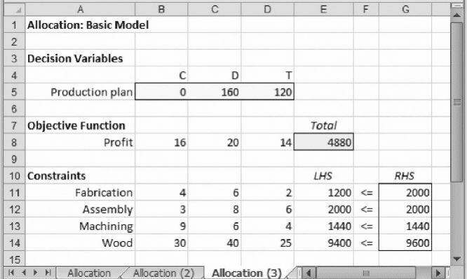
Figure 2.6 displays the optimal solution to our model for the example.
†
The optimal plan contains no chairs, 160 desks, and 120 tables.
†
The maximum profit contribution is $4880.
†
The binding constraints are assembly capacity and machining capacity.
These are the three key pieces of information provided in the solution. Evidently,
the profit margin on chairs is not sufficiently attractive for us to devote scarce resources
to their production. But even by relying on desks and tables, Brown Furniture can
maximize its profit contribution for the month. (We examine the solution in more
detail later on.)
Recall the distinction made earlier between tactical and strategic information in
the linear program’s solution. Faced with implementing a production plan for next
month at Brown Furniture, we could pursue the tactical solution, producing no
chairs, 160 desks, and 120 tables. However, the tactical solution is the optimal solution
Figure 2.5. Specifications on the Engine tab.
34 Chapter 2 Linear Programming: Allocation, Covering, and Blending Models
for the model. Perhaps it is not the optimal solution for the actual problem facing
Brown Furniture. For example, a relevant marketing consideration might have been
omitted from the model. Perhaps our marketing department is reluctant to bring a lim-
ited product line to the marketplace—that is, by producing no chairs at all. Even if the
optimization of a short-term objective calls for a limited product line, long-term risks
may arise if some customers conclude that Brown Furniture cannot make chairs. Thus,
the optimal solution of the model may turn out to be only the first step in a discussion
of how to reflect long-term marketing needs in short-term planning processes.
Possibly, this discussion will lead to revisions in the model, and the optimal solution
will be revisited.
On the other hand, if there were time to adjust the resources available at Brown
Furniture and we were interested in the strategic implications of the solution, we
would want to explore the possibility of acquiring more assembly capacity or machin-
ing capacity because those are the binding constraints. We know that additional fab-
rication capacity or wood supply would not provide any benefit, given current
conditions, because we can achieve optimal profits without fully consuming either
of those resources. Overcoming the limited supply of assembly capacity and machin-
ing capacity is the key to achieving higher profits.
2.2.1. The Product Mix Problem
The product mix problem is a variation of the basic allocation model. It follows the
structure of the allocation model by prescribing the maximization of profit contri-
bution subject to LT constraints. Typically, the decision variables correspond to quan-
tities of various products to include in a company’s product mix. The constraints are
Figure 2.6. Optimal solution to the Brown Furniture model.
2.2. Allocation Models 35