Balakumar Balachandran, Magrab E.B. Vibrations
Подождите немного. Документ загружается.

6.4 RESPONSE TO RAMP INPUT
We now consider the response of a linear vibratory system to a ramp input and
we use this response to demonstrate the effects of rise time of the input force
on the rise time and overshoot of the response x(t). The ramp waveform,
which is shown in Figure 6.17, is described by
(6.34) F
o
for
t t
o
F
o
t
t
o
for
0 t t
o
f 1t 2 0 for
t 0
310 CHAPTER 6 Single Degree-of-Freedom Systems Subjected to Transient Excitations
Time domain Frequency domain
0 0.5 1 1.5
0.6
0.5
0.4
0.3
0.2
0.1
0
0.1
0.2
0.3
t (s)
a
c
(t)a
c
(t)
a
o
0.15 m/s
2
a
o
0.6 m/s
2
a
o
0.15 m/s
2
a
o
0.6 m/s
2
a
o
0.15 m/s
2
a
o
0.6 m/s
2
(a)
0 2 4 6 8 10
12
0
0.05
0.1
0.15
0.2
0.25
Frequency (Hz)
|a
cs
( j
v
)|
|a
cs
( j
v
)|
a
o
0.15 m/s
2
a
o
0.6 m/s
2
(b)
(c)
0 2 4 6 8 10 12
0
0.05
0.1
0.15
0.2
0.25
Frequency (Hz)
(d)
0 0.5 1 1.5
t (s)
0.6
0.5
0.4
0.3
0.2
0.1
0
0.1
0.2
0.3
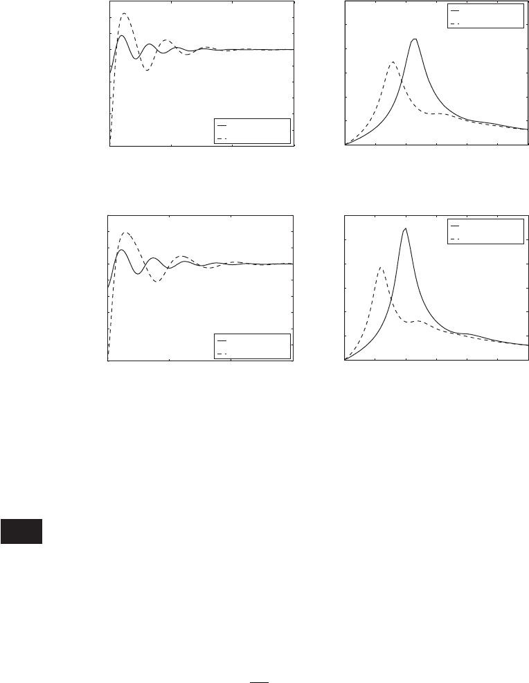
FIGURE 6.16
Time and frequency responses of car seat to step acceleration inputs: (a) and (b) M 36 kg and (c) and (d) M 45 kg.

When the ramp input approaches a step input. From Eqs. (6.30) and
(6.34), we find that the rise time of the ramp portion of the forcing is
Equation (6.34) is written in terms of the unit step function as
(6.35)
Referring to Figure 6.16, we see that Eq. (6.35) is the sum of two ramps
f
1
(t) and f
2
(t) whose slopes are the negative of each other’s slope and which
are time shifted with respect to each other by an amount t
o
. In terms of non-
dimensional time t, Eq. (6.35) is rewritten as
(6.36)
where After substituting Eq. (6.36) into Eq. (6.1b), and defining
the following quantity
we determine the response of the system given in Figure 6.1 as
14
F
o
t
o
k21 z
2
cu1t2
t
0
g1t,j 2jdj u1t t
o
2
t
t
o
g1t,j 21j t
o
2dj d
x 1t2
F
o
t
o
k21 z
2
c
t
0
g1t,j 2ju1j2dj
t
0
g1t,j 21j t
o
2u1j t
o
2dj d
g1t,j 2 e
z1tj2
sin a1t j221 z
2
b
t
o
v
n
t
o
.
f 1t2
F
o
t
o
3tu1t2 1t t
o
2u1t t
o
24
F
o
t
o
3tu1t2 1t t
o
2u1t t
o
24
f 1t 2 F
o
c
t
t
o
3u1t2 u1t t
o
24 u1t t
o
2d
t
r
0.8t
o
.
t
o
씮 0,
6.4 Response to Ramp Input 311
14
In these equations, the unit step function determines the lower limit of integration. In addition,
we must also place the unit step function outside the integrals to explicitly indicate the regions of
applicability of each integral as a function of t.
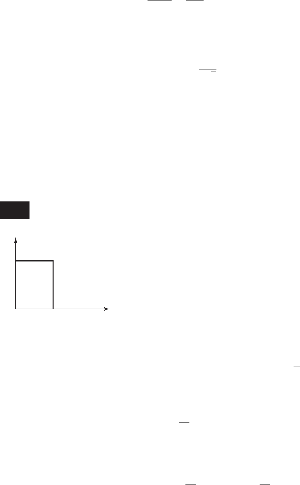
f(t)
F
o
t
o
t
f
1
(t) f
2
(t)
F
o
F
o
t
o
t
o
2t
o
t
t
0
0
FIGURE 6.17
Ramp force composed of two ramps.

Shifting the time variable in the second integral, we rewrite the above
expression as
since
After performing the integration, we obtain
(6.37)
where the first term on the right-hand side of Eq. (6.37) is the response to the
ramp function f
1
(t) given by the first term of Eq. (6.36) and the second term
on the right-hand side is the response to the ramp function f
2
(t) given by the
second term of Eq. (6.36). The function h(t) is given by
(6.38)
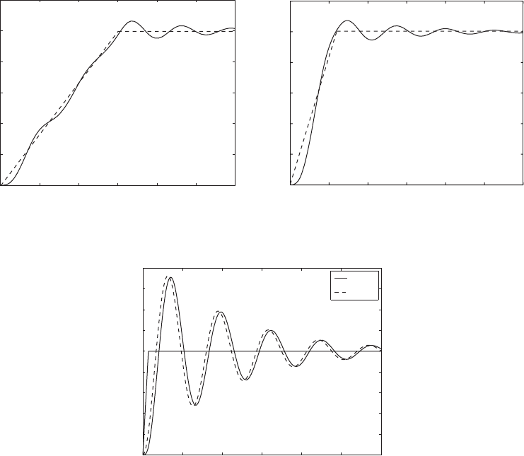
The displacement response given by Eq. (6.37) is plotted in Figure 6.18,
where it is seen that as the rise time of the ramp input decreases, the amount
of overshoot increases and the displacement response deviates more from the
input waveform. For comparison, the response to a step input is also included
in Figure 6.18c. As the rise time of the ramp becomes shorter, the response
closely resembles the response to a step input of corresponding magnitude.
Also, from Eqs. (6.37) and (6.38), it is noticed that as z increases, the over-
shoot decreases.
2z
2
1
21 z
2
sin at21 z
2
bdf
h1t 2
1
t
o
e2z t e
zt
c2z cos at 21 z
2
b
x 1t2
F
o
k
3h1t2u1t 2 h1t t
o
2u1t t
o
24
g1t t
o
,j2
e
z1tt
o
j2
sin a1t t
o
j221 z
2
b
g1t,j t
o
2 e
z1t3jt
o
42
sin a1t 3j t
o
4221 z
2
b
F
o
t
o
k21 z
2
cu1t2
t
0
g1t,j 2jdj u1t t
o
2
tt
o
0
g1t t
o
,j2jdj d
x 1t2
F
o
t
o
k21 z
2
cu1t2
t
0
g1t,j 2jdj u1t t
o
2
tt
o
0
g1t,j t
o
2jdj d
312 CHAPTER 6 Single Degree-of-Freedom Systems Subjected to Transient Excitations
6.4 Response to Ramp Input 313
x(t)/(F
o
/k)
0
0.2
0.4
0.6
0.8
1
1.2
1.4
1.6
1.8
Ramp
Step
(c)
0 5 10 15 20 25 30
t
0 5 10 15 20 25 30
0
0.2
0.4
0.6
0.8
1
1.2
t
x(t)/(F
o
/k)
x(t)/(F
o
/k)
(a)
(b)
0510
15
20 25 30
t
0
0.2
0.4
0.6
0.8
1
1.2
FIGURE 6.18
Response of system to the ramp force given in Figure 6.17 for z 0.1 and different rise times: (a) t
o
v
n
t
o
15; (b) t
o
v
n
t
o
6;
and (c) t
o
v
n
t
o
0.7. In (a) and (b), the broken line is used to represent the input and the solid line is used to represent the
response.
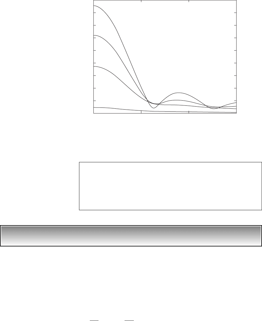
The maximum displacement response x
max
, which is a function of
the ramp duration t
o
and the damping factor z, is determined numerically
15
based on Eqs. (6.37) and (6.38). The results are shown in Figure 6.19. For
minimum values of x
max
occur in the vicinity of t
o
2p,4p, ..,
which are multiples of the period of the system’s natural frequency. Hence,
we can propose the following design guideline to decrease a system’s
overshoot.
z 0.015,
15
The MATLAB function fminbnd from the Optimization Toolbox was used.
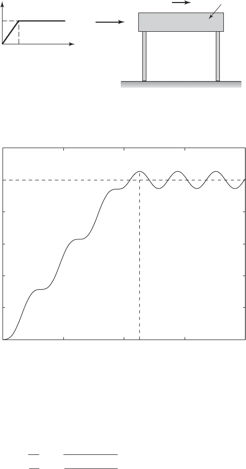
EXAMPLE 6.7 Response of a slab floor to transient loading
Consider the vibratory model of a slab floor shown in Figure 6.20. The slab
floor has a mass of 1000 kg and the equivalent stiffness of each column sup-
porting the system is 2 10
5
N/m. The transient loading f(t) acting on the
floor has the amplitude versus time profile shown in Figure 6.20. We shall
determine the response x(t) of the slab floor and find the earliest time at which
the maximum response occurs.
The governing equation of motion of the system is given by Eq. (3.22)
with z 0. Thus,
(a)
d
2
x
dt
2
v
n
2
x
f 1t 2
m
314 CHAPTER 6 Single Degree-of-Freedom Systems Subjected to Transient Excitations
1.9
1.8
1.7
1.6
1.5
1.4
1.3
1.2
1.1
1
0
x
max
/(F
o
/k)
510
o
0.05
0.15
0.3
0.7
15
FIGURE 6.19
Maximum displacement of single degree-of-freedom system to ramp forcing shown in
Figure 6.17 for several different damping factors.
Design Guideline: Either increasing damping of a vibratory system
or increasing the rise time of the external forcing function can decrease
the amount of overshoot in the response of a single degree-of-freedom
system subjected to a ramp excitation. In addition, for systems with
the overshoot has minima at t
o
2np, n 1, 2, ...z 0.015,
where
(b)
Making use of Eq. (6.35), the forcing function is written as
(c)
10003tu1t 2 1t 12u1t 1 24
N
f 1t 2 10005t 3u1t 2 u1t 124 u1t 1 26 N
v
n
B
2k
m
B
2 2 10
5
1000
20 rad/s
6.4 Response to Ramp Input 315
f(t)
f(t)
1
t (s)
x(t)
1000 N
k
m
k
Floor slab
FIGURE 6.20
Floor slab subjected to ramp forcing.
FIGURE 6.21
Response of the floor slab shown in Figure 6.20.
0 0.5 1 1.5 2
0
0.5
1
1.5
2
2.5
3
x(t) (mm)
t (s)
x
max
t
max

To determine the response x(t), we first recognize that in Eq. (6.38)
Also, z 0 because we have an undamped system.
Then,
(d)
Then, from Eq. (6.37), the displacement response of the slab is given by
(e)
where we have used the fact that F
o
/k 1000/410
5
m 2.5 10
3
m
2.5 mm. A graph of Eq. (e) is shown in Figure 6.21. The earliest time
at which the maximum value x(t) is found numerically
16
to be x
max
2.64 mm at t
m
1.13 s.
6.5
SPECTRAL ENERGY OF THE RESPONSE
The total energy E
T
in a signal g(t), which has a Laplace transform G(s), is
17
(6.39)
which, by Parseval’s theorem,
18
is also given by
(6.40)
where |G( jv)|
2
is the energy density spectrum with units (E
u
2
s)/rad/s, E
u
has
the physical or engineering unit of g(t); that is, it represents N, Pa, m/s, etc.,
and |G( jv)| is the amplitude density spectrum with the units E
u
/rad/s. Hence,
from either Eq. (6.39) or Eq. (6.40), the energy associated with a signal g(t)
can be determined. Typically, the signals of interest will be the displacement
response x(t) and the forcing f(t).
The energy over a portion of the frequency range 0 v v
c
is deter-
mined from
(6.41)E1v
c
2
1
p
v
c
0
|G1jv2|
2
dv
E
T
1
p
q
0
|G1jv2|
2
dv
E
T
q
0
g
2
1t 2dt
0.05 sin120 3t 1426u1t 1 24 mm
x 1t 2 2.535t 0.05 sin120t 26u1t 2 51t 1 2
h1t 2
1
v
n
5v
n
t sin1v
n
t26 t 0.05 sin120t2
t v
n
t and t
o
v
n
.
316 CHAPTER 6 Single Degree-of-Freedom Systems Subjected to Transient Excitations
16
The MATLAB function fminbnd from the Optimization Toolbox was used.
17
For this equation to be valid, the signal must be bounded and its energy must be finite.
18
See, for example, Papoulis, ibid., p. 27 ff.
The fraction of total energy in this frequency band can be written as
(6.42)
If v
c
is the cutoff frequency of the amplitude density spectrum, then v
c
is determined from the relation
(6.43)
where is the maximum value of |G( jv)|, which occurs at v
max
and 0 v
max
v
c
.
In the next two sections, we shall develop relationships among the cutoff
frequency v
c
, the rise time t
r
, the fraction of total energy in the region
0 v v
c
, and the effect of
c
v
c
/v
n
on the system’s displacement re-
sponse as a function of time for different pulse excitations. This information
is useful for the design of components subjected to shock excitations, which
are typically modeled as pulse excitations.
6.6 RESPONSE TO RECTANGULAR PULSE EXCITATION
We now consider the application of a force whose time profile is rectangular,
as shown in Figure 6.22. In terms of the unit step function, this force is rep-
resented by
(6.44)
Then, by using Eqs. (6.39) and (6.44), the total energy in the pulse is
(6.45)
Note that for the total energy in the pulse to remain constant, either F
o
or t
o
has to be adjusted so that F
o
varies as By using the Laplace transform
pair 8 in Table A in Appendix A, the Laplace transform of f(t) given by
Eq. (6.44) is
(6.46)
We obtain the associated amplitude spectrum and phase spectrum by
making the substitution s jv into Eq. (6.46). This results in
(6.47) G
r
1v 2e
jc1v2
F1jv2
F
o
jv
11 e
jvt
o
2
F
o
v
3sin vt
o
j1cos vt
o
124
F1s 2
F
o
s
11 e
st
o
2
2t
o
.
E
T
t
o
0
F
o
2
dt F
o
2
t
o
f 1t2 F
o
3u1t2 u1t t
o
24
0G1jv20
v v
max
0G1jv
c
20
1
22
0G1jv20
v v
max
E1v
c
2
E
T
1
E
T
p
v
c
0
0G1jv20
2
dv
6.6 Response to Rectangular Pulse Excitation 317
f
(t)
F
o
t
o
t
FIGURE 6.22
Rectangular force pulse.
318 CHAPTER 6 Single Degree-of-Freedom Systems Subjected to Transient Excitations
where the pulse amplitude function G
r
(v) and the pulse phase function c(v)
are given by
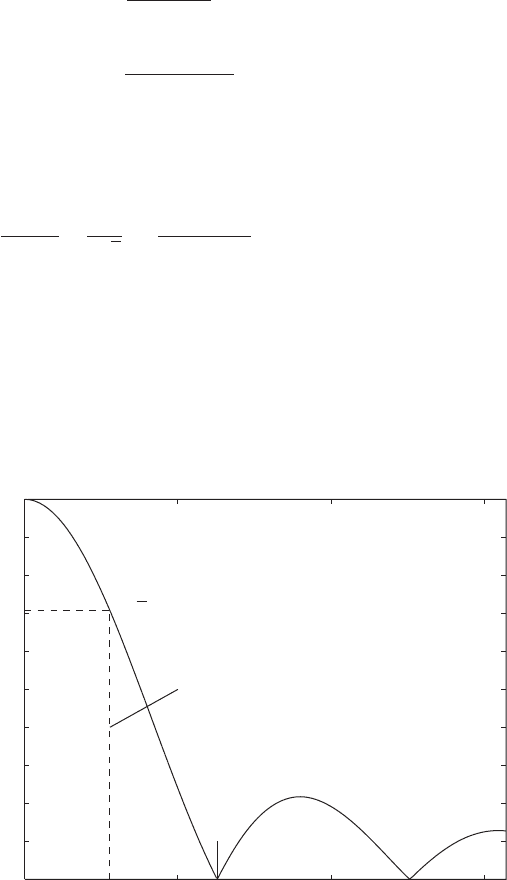
(6.48)
The quantity G
r
(v)/(F
o
t
o
) is plotted in Figure 6.23.
Hence, from Eqs. (6.48), the cutoff frequency v
c
associated with the
input force spectrum is determined from the numerical solution to
which gives
19
(6.49)
We call c
r
the pulse duration–bandwidth product; thus, as the pulse duration
t
o
decreases, the bandwidth v
c
increases proportionately.
c
r
v
c
t
o
2.7831
G
r
1v
c
2
F
o
t
o
1
22
2
sin 1v
c
t
o
/2 2
v
c
t
o
/2
2
c1v 2 tan
1
cos1vt
o
2 1
sin1vt
o
2
tan
1
1tan1vt
o
/2 22vt
o
/2
G
r
1v 2 F
o
t
o
2
sin1vt
o
/2 2
vt
o
/2
2
19
The MATLAB function fzero was used.
0 5 10 15
0
0.1
0.2
0.3
0.4
0.5
0.6
0.7
0.8
0.9
1
vt
o
G
r
(v)/(F
o
t
o
)
2p
1/
√
2
v
c
t
o
2.783
FIGURE 6.23
Normalized amplitude spectrum of rectangular pulse of duration t
o
.

From Eq. (6.42), the fraction of the total energy in the frequency range
is
(6.50)
where the integral was evaluated numerically.
20
We see that 72.2% of the to-
tal energy of the rectangular pulse lies within this bandwidth. In addition, it is
numerically found that E(2p)/E
T
0.903, or about 90% of the energy of the
rectangular pulse lies in the bandwidth 0 v 2p/t
o
.
The amplitude spectrum and the phase spectrum of the displacement re-
sponse of the mass are determined from Eqs. (5.55), (6.19), and (6.47). Thus,
(6.51)
where the response amplitude function X(v) and the response phase function
f(v) are given by
(6.52)
where u(v) is given by Eq. (5.56b) and c(v) is given by Eq. (6.48).
In order to be able to make comparisons for various combinations of pa-
rameters, we introduce notations in terms of E
T
, the total energy of the applied
orce, and v
c
, the cutoff frequency. To have valid comparisons, we have chosen
the total energy to be the same in all cases. We also want to be able to deter-
mine the effects of the cutoff frequency of the applied pulse in terms of the
natural frequency of the system. To this end, we introduce the following
notation
(6.53)
Then, Eq. (6.52) is written as
(6.54)
X
r
1v 2
E
1
/k
1
2
c
211
2
2
2
12z2
2
2
sin1c
r
/2
c
2
c
r
/2
c
2
F
o
t
o
k
E
1
k2
c
F
o
k
E
o
2
c
k
v/v
n
c
v
c
/v
n
E
1
B
c
r
E
T
v
n
E
o
B
E
T
v
n
c
r
f1v 2 u1v 2 c1v2
X
r
1v 2
F
o
t
o
k211 1v/v
n
2
2
2
2
12zv/v
n
2
2
2
sin1vt
o
/2 2
vt
o
/2
2
X1jv2 G1jv 2F1jv2 X
r
1v2e
jf1v2
E1v
c
t
o
2
E
T
1
p
v
c
t
o
0
`
sin1x/22
x/2
`
2
dx 0.722
0 v v
c
6.6 Response to Rectangular Pulse Excitation 319
20
The MATLAB function trapz was used.