Balakumar Balachandran, Magrab E.B. Vibrations
Подождите немного. Документ загружается.

This equation has been rewritten as the first of Eqs. (7.1a). Similarly, from the
free-body diagram of inertial element m
2
, the second of Eqs. (7.1a) is
obtained.
(7.1a)
These linear differential equations are written in matrix form
1
as
(7.1b)
The off-diagonal terms of the inertia matrix are zero, while the off-diagonal
terms of the stiffness and damping matrices are non-zero. In addition, all of
these matrices are symmetric matrices.
2
The equations governing the system
are coupled due to these non-zero off-diagonal terms in the stiffness and
damping matrices. Physically, the system is uncoupled when the damper c
2
and the spring k
2
are absent. The excitations f
1
(t) and f
2
(t) are directly applied
to the inertial elements of the system as shown in the figure.
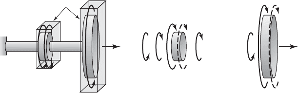
Moment-Balance Method
We now consider the system shown in Figure 7.3, which has two flywheels
with rotary inertias J
o1
and J
o2
. The end of the shaft attached to the rotor is
treated as a fixed end. The drive torque to the first flywheel is M
o
(t). The gen-
eralized coordinates f
1
and f
2
are used to describe the rotations of the fly-
wheels about the axis k through the respective centers. The inertias of the
shafts are neglected, the torsional stiffness of the shaft in between the fixed
end and the flywheel closest to it is represented by k
t1
, and the torsional
c
k
1
k
2
k
2
k
2
k
2
k
3
de
x
1
x
2
f e
f
1
f
2
f
c
m
1
0
0 m
2
de
x
$
1
x
$
2
f c
c
1
c
2
c
2
c
2
c
2
c
3
de
x
#
1
x
#
2
f
m
2
x
$
2
1c
2
c
3
2x
#
2
c
2
x
#
1
1k
2
k
3
2x
2
k
2
x
1
f
2
1t 2
m
1
x
$
1
1c
1
c
2
2x
#
1
c
2
x
#
2
1k
1
k
2
2x
1
k
2
x
2
f
1
1t 2
340 CHAPTER 7 Multiple Degree-of-Freedom Systems
1
See Appendix E for a brief introduction to matrix notation.
2
As discussed in Appendix E, a matrix [A] is called a symmetric matrix if the elements of the
matrix a
ij
a
ji
.
FIGURE 7.3
(a) System of two flywheels driven by a rotor and (b) free-body diagrams along with the
respective inertial moments illustrated by broken lines.
(a) (b)
k
t1
1
2
k
t2
kk
J
o1
J
o2
M
o
(t)
M
o
(t)
Oil housing
k
t1
1
c
t1
1
J
o1
1
k
t2
(
1
2
)
.
c
t2
2
.
..
J
o2
2
..

stiffness of the other shaft is represented by k
t2
. It is assumed that the fly-
wheels are immersed in housings filled with oil and that the corresponding
dissipative effect is modeled by using the viscous damping coefficients c
t1
and
c
t2
. In the free-body diagrams of Figure 7.3, the inertial moments
and are also shown.
Based on the free-body diagrams shown in Figure 7.3, we apply the prin-
ciple of angular momentum balance to each of the flywheels and obtain the
governing equations
(7.2a)
which are written in matrix form as
(7.2b)
In this case, the equations are coupled because of the non-zero off-diagonal
terms in the stiffness matrix, which are due to the shaft with stiffness k
t2
.
Both of the physical systems chosen for illustration of force-balance and
moment-balance methods are described by linear models and the associated
governing system of equations is written in matrix form. This is possible to
do for any linear multi-degree-of-freedom system, as illustrated in Example
7.1. For a nonlinear multi-degree-of-freedom system, the governing nonlin-
ear equations of motion are linearized to obtain a set of linear equations; the
resulting linear equations are amenable to matrix form. This is illustrated in
Example 7.3.
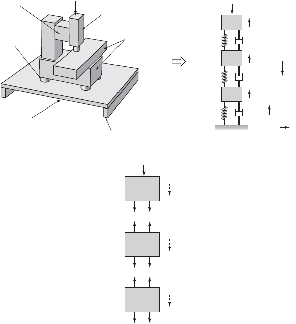
EXAMPLE 7.1
Modeling of a milling machine on a flexible floor
A milling machine and a vibratory model of this system are shown in Fig-
ure 7.4. We shall derive the governing equations of motion for this system by
using the force-balance method. As shown in Figure 7.4b, the milling ma-
chine is described by using the three inertial elements m
1
, m
2
, and m
3
along
with discrete spring elements and damper elements. All three inertial ele-
ments translate only along the i direction. The external force f
1
(t) in the i di-
rection shown in the figure is a representative disturbance acting on m
1
.
To obtain the governing equations of motion, we use the generalized co-
ordinates x
1
, x
2
, and x
3
, each measured from the system’s static equilibrium
position. Since the coordinates are measured from the static equilibrium po-
sition, gravity forces are not considered below. In order to apply the force-
balance method to each inertial element, the free-body diagrams shown in
Figure 7.4c are used. Applying the force-balance method along the i direction
to each of the masses, we obtain the following equations:
(a)m
3
x
$
3
1k
2
k
3
2x
3
k
2
x
2
1c
2
c
3
2x
#
3
c
2
x
#
2
0
m
2
x
$
2
1k
1
k
2
2x
2
k
1
x
1
k
2
x
3
1c
1
c
2
2x
#
2
c
1
x
#
1
c
2
x
#
3
0
m
1
x
$
1
k
1
1x
1
x
2
2 c
1
1x
#
1
x
#
2
2f
1
1t 2
c
J
o1
0
0 J
o2
de
f
$
1
f
$
2
f c
c
t1
0
0 c
t2
de
f
#
1
f
#
2
f c
k
t1
k
t2
k
t2
k
t2
k
t2
de
f
1
f
2
f e
M
o
1t 2
0
f
J
o2
f
$
2
c
t2
f
#
2
k
t2
1f
2
f
1
2 0
J
o1
f
$
1
c
t1
f
#
1
k
t1
f
1
k
t2
1f
1
f
2
2 M
o
1t 2
J
o2
f
$
2
k
J
o1
f
$
1
k
7.2 Governing Equations 341
342 CHAPTER 7 Multiple Degree-of-Freedom Systems
FIGURE 7.4
(a) Milling machine; (b) vibratory model for study of vertical motions; and (c) free-body dia-
grams of inertial elements m
1
, m
2
, and m
3
shown in (b) along with the inertial forces illustrated
by broken lines.
Equations (a) are arranged in the following matrix form:
(b)
We see that the inertia, the stiffness, and the damping matrices are symmetric
matrices.
£
k
1
k
1
0
k
1
k
1
k
2
k
2
0 k
2
k
2
k
3
§•
x
1
x
2
x
3
¶ •
f
1
1t 2
0
0
¶
C
m
1
00
0 m
2
0
00m
3
S•
x
$
1
x
$
2
x
$
3
¶ C
c
1
c
1
0
c
1
c
1
c
2
c
2
0 c
2
c
2
c
3
S•
x
#
1
x
#
2
x
#
3
¶
k
2
x
1
(t)
x
2
(t)
x
3
(t)
x
g
y
c
1
c
2
c
3
k
1
k
3
m
1
m
2
m
3
m
1
(b)(a)
Machine tool head, m
1
Machine tool base, m
2
(c)
j
i
f
1
(t)
f
1
(t)
m
1
x
1
k
1
(x
1
– x
2
) c
1
(x
1
– x
2
)
..
m
2
x
2
..
m
3
x
3
..
..
c
2
(x
2
– x
3
)
..
m
2
k
2
(x
2
– x
3
)
m
3
k
3
x
3
c
3
x
3
.
Rigid floor support
Flexible support, k
1
Elastic mount, k
2
Floor, m
3
and k
3
f
1
(t)

EXAMPLE 7.2 Conservation of linear momentum in a multiple
degree-of-freedom system
We revisit Example 7.1 and discuss when the linear momentum of this
multiple degree-of-freedom system is conserved along the i direction. From
Eq. (1.11), it is clear that in the absence of external forces f
i
(t), the linear mo-
mentum of the system is conserved; that is,
(a)
Even in the absence of the forcing f
1
(t) in Example 7.1, the linear momentum
of this three degree-of-freedom system is not conserved because of the forces
acting at the base of the system. To examine this, we set f
1
(t) = 0 in Eq. (a) of
Example 7.1 and arrive at the following equations:
(b)
Each of Eqs. (b) was obtained by performing a linear-momentum balance in-
dividually for each of the three inertial elements of the system. Adding all
three equations of Eqs. (b), we obtain
(c)
Integrating Eq. (c) with respect to time—that is,
(d)
—leads to
(e)
From Eq. (e), it follows that due to the presence of the spring and damper
forces at the base, the total linear momentum of the system is not conserved.
If the spring with stiffness k
3
and the damper with damping coefficient c
3
were
absent, then the total linear momentum of the resulting free-free system is
conserved.
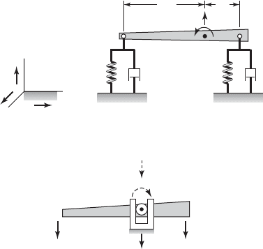
EXAMPLE 7.3
System with bounce and pitch motions
Consider the rigid bar shown in Figure 7.5a, which can rotate (pitch) about
the k direction and translate (bounce) along the j direction. We locate the gen-
eralized coordinates y and u at the center of gravity of the beam. This model
m
1
x
#
1
m
2
x
#
2
m
3
x
#
3
constant
t
0
1m
1
x
$
1
m
2
x
$
2
m
3
x
$
3
2dt
t
0
1k
3
x
3
c
3
x
#
3
2dt
m
1
x
$
1
m
2
x
$
2
m
3
x
$
3
1k
3
x
3
c
3
x
#
3
2
m
3
x
$
3
1k
2
k
3
2x
3
k
2
x
2
1c
2
c
3
2x
#
3
c
2
x
#
2
0
m
2
x
$
2
1k
1
k
2
2x
2
k
1
x
1
k
2
x
3
1c
1
c
2
2x
#
2
c
1
x
#
1
c
2
x
#
3
0
m
1
x
$
1
k
1
1x
1
x
2
2 c
1
1x
#
1
x
#
2
2 0
dp
dt
0
씮
p constant
7.2 Governing Equations 343
provides a good representation for describing certain types of motions of mo-
torcycles, automobiles, and other vehicles.
This particular example has been chosen to illustrate that both the force-
balance and moment-balance methods are needed to obtain the governing
equations. In addition, we also illustrate how the equilibrium positions are de-
termined and how linearization of a nonlinear system is carried out.
Governing Equations of Motion
The free-body diagram shown in Figure 7.5b will be used to obtain the gov-
erning equations of motion. The inertial force and the inertial moment are also
shown in Figure 7.5b. Considering force balance and moment balance with
respect to the center of mass G of the rigid bar, we obtain, respectively,
(a)
and
(b)
Equations (a) and (b) are nonlinear because of the sin u and cos u terms.
1k
1
L
1
k
2
L
2
2y cos u 1k
1
L
1
2
k
2
L
2
2
2sin u cos u 0
J
G
u
$
1c
1
L
1
c
2
L
2
2y
#
cos u 1c
1
L
1
2
c
2
L
2
2
2u
#
cos
2
u
1k
1
L
1
k
2
L
2
2sin u mg
my
$
1c
1
c
2
2y
#
1c
1
L
1
c
2
L
2
2u
#
cos u 1k
1
k
2
2y
344 CHAPTER 7 Multiple Degree-of-Freedom Systems
FIGURE 7.5
(a) Rigid body in the plane constrained by springs and dampers and (b) free-body diagram of the
system along with the inertial force and the inertial moment.
my
k
2
(y L
2
sin )
c
2
(y L
2
cos )
k
1
(y L
1
sin )
c
1
(y L
1
cos )
k
1
k
2
c
1
L
1
L
2
c
2
i
x
y
y
z
j
k
(a)
(b)
.
.
.
.
..
..
G
G
m, J
G
mg
J
G

Static-Equilibrium Positions
The equilibrium positions y
o
and u
o
of the system are obtained by setting the
accelerations and velocities to zero in Eqs. (a) and (b). Thus, y
o
and u
o
are so-
lutions of
(c)
From the second of Eqs. (c), we find that
(d)
Making use of the second of Eqs. (d) in the first of Eqs. (c), we arrive at
(e)
Note that the equilibrium position u
o
p/2 corresponding to cos u
o
0 in
Eqs. (d) is not considered because it is not physically meaningful. Examining
Eq. (e), y
o
represents a sag in the position of the bar due to the weight of the
bar. From the second of Eqs. (d), u
o
represents a rotation due to the combina-
tion of the unequal stiffness at each end and the unequal mass distribution of
the bar. When k
1
L
1
k
2
L
2
, u
o
0, but y
o
0. For k
1
L
1
k
2
L
2
, in the absence
of gravity loading or other constant loading, y
o
0, and hence, u
o
0.
Linearization and Linear System Governing “Small” Oscillations
about an Equilibrium Position
We now consider “small” oscillations of the system shown in Figure 7.5 about
the equilibrium position (y
o
, u
o
). In order to obtain the governing equations,
we substitute
(f)
into Eqs. (a) and (b) and carry out Taylor-series expansions
3
of sin u and cos u,
and retain the linear terms in y and u. To this end, we find that
(g)cosu cos 1u
o
u
ˆ
2 cosu
o
u
ˆ
sinu
o
. . .
sin u sin1u
o
u
ˆ
2 sin u
o
u
ˆ
cos u
o
. . .
u
$
1t 2
d
2
dt
2
1u
o
u
ˆ
2 u
ˆ
$
1t 2,
u
#
1t 2
d
dt
1u
o
u
ˆ
2 u
ˆ
#
1t 2
y
$
1t 2
d
2
dt
2
1y
o
y
ˆ
2 y
ˆ
$
1t 2,
y
#
1t 2
d
dt
1y
o
y
ˆ
2 y
ˆ
#
1t 2
u1t 2 u
o
u
ˆ
1t 2
y1t 2 y
o
y
ˆ
1t 2
y
o
mg1k
1
L
1
2
k
2
L
2
2
2
k
1
k
2
1L
1
L
2
2
2
cos u
o
0
or
sin u
o
y
o
1k
1
L
1
k
2
L
2
2
1k
1
L
1
2
k
2
L
2
2
2
531k
1
L
1
k
2
L
2
2y
o
1k
1
L
1
2
k
2
L
2
2
2sin u
o
46cos u
o
0
1k
1
k
2
2y
o
1k
1
L
1
k
2
L
2
2sin u
o
mg
7.2 Governing Equations 345
3
T. B. Hildebrand, ibid.
On substituting Eqs. (g) into Eqs. (a) and (b), making use of Eqs. (c), and re-
taining only the linear terms in and , we arrive at
(h)
which in matrix form reads as
(i)
Equation (i) represents the linear system governing “small” oscillations of the
system shown in Figure 7.5 about the static equilibrium position given by
Eqs. (d) and (e). Although the gravity loading determines the equilibrium po-
sition, it does not appear explicitly in Eq. (i). Hence, when it is assumed that
the generalized coordinates are measured from the static-equilibrium posi-
tion, constant loading such as gravity loading is not considered for determin-
ing the equations of motion.
From the second of Eqs. (d) it is seen that if k
1
L
1
k
2
L
2
, u
o
0, and
Eq. (i) takes the form
(j)
If k
1
L
1
k
2
L
2
and u
o
0, then Eq. (i) takes the form
(k)
When c
1
L
1
c
2
L
2
and k
1
L
1
k
2
L
2
the equations uncouple: that is, the rota-
tion and translation motions of the bar are independent of each other.
It is noted that Eqs. (k) could have been obtained directly, if it had been
initially assumed that “small” oscillations about the static-equilibrium posi-
tion were being considered and that the static-equilibrium position is “close”
to the horizontal position. In this case, cos u would have been set to 1 and sin u
would have been replaced by u in Eqs. (a) and (b).
c
k
1
k
2
1k
1
L
1
k
2
L
2
2
1k
1
L
1
k
2
L
2
21k
1
L
1
2
k
2
L
2
2
2
de
y
ˆ
u
ˆ
f e
0
0
f
c
m 0
0 J
G
de
yˆ
$
u
ˆ
$
f c
c
1
c
2
1c
1
L
1
c
2
L
2
2
1c
1
L
1
c
2
L
2
21c
1
L
1
2
c
2
L
2
2
2
de
yˆ
#
u
ˆ
#
f
c
k
1
k
2
0
0 1k
1
L
1
2
k
2
L
2
2
2
de
y
ˆ
u
ˆ
f e
0
0
f
c
m 0
0 J
G
de
yˆ
$
u
ˆ
$
f c
c
1
c
2
1c
1
L
1
c
2
L
2
2
1c
1
L
1
c
2
L
2
21c
1
L
1
2
c
2
L
2
2
2
de
yˆ
#
u
ˆ
#
f
c
k
1
k
2
1k
1
L
1
k
2
L
2
2cos u
o
1k
1
L
1
k
2
L
2
2cos u
o
1k
1
L
1
2
k
2
L
2
2
21cos
2
u
o
sin
2
u
o
2
de
y
ˆ
u
ˆ
f e
0
0
f
c
m 0
0 J
G
de
y
ˆ
$
u
ˆ
$
f c
c
1
c
2
1c
1
L
1
c
2
L
2
2cosu
o
1c
1
L
1
c
2
L
2
2cosu
o
1c
1
L
1
2
c
2
L
2
2
2cos
2
u
o
de
y
ˆ
#
u
ˆ
#
f
1k
1
L
1
k
2
L
2
2y
ˆ
cos u
o
1k
1
L
1
2
k
2
L
2
2
2u
ˆ
1cos
2
u
o
sin
2
u
o
2 0
J
G
u
ˆ
$
1c
1
L
1
c
2
L
2
2y
ˆ
#
cos u
o
1c
1
L
1
2
c
2
L
2
2
2u
ˆ
#
cos
2
u
o
1k
1
L
1
k
2
L
2
2u
ˆ
cos u
o
0
my
ˆ
$
1c
1
c
2
2y
ˆ
#
1c
1
L
1
c
2
L
2
2u
ˆ
#
cos u
o
1k
1
k
2
2y
ˆ
u
ˆ
y
ˆ
346 CHAPTER 7 Multiple Degree-of-Freedom Systems
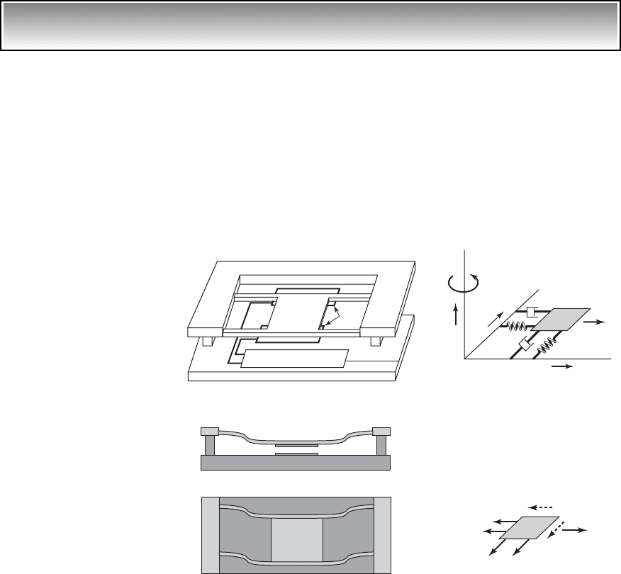
EXAMPLE 7.4 Governing equations of a rate gyroscope
4
We shall obtain the governing equations of motion of a rate gyroscope, also
known as a gyro-sensor. The physical system, along with the vibratory model,
is shown in Figure 7.6. In the vibratory model shown in Figure 7.6b, the sen-
sor is shown as a point mass m with two degrees of freedom and its motion is
described by the coordinates x and y in the horizontal plane. The generalized
coordinates are both located in a rotating reference frame. The sensor is to be
designed to measure the rotational speed v
z
, which is assumed constant. For
modeling purposes, a spring with stiffness k
x
and a viscous damper with a
damping coefficient c
x
are used to constrain motions along the n
1
direction.
7.2 Governing Equations 347
4
O. Degani, D. J. Seter, E. Socher, S. Kaldor, and Y. Nemirovsky, “Optimal Design and Noise
Consideration of Micromachined Vibrating Rate Gyroscope with Modulated Integrative Differ-
ential Optical Sensing,” J. Microelectromechanical Systems, Vol. 7, No. 3, pp. 329–338 (1998).
FIGURE 7.6
(a) Micromachined rate gyroscope; (b) vibratory model; and (c) free-body diagram along with
the inertial forces. [(1) Suspended proof mass; (2) frame; (3) CMOS chip; (4) photodiodes; and
(5) electronic circuitry.] Source: Fig. 7.6a from O. Degani, D. J. Seter, E. Socher, S. Kaldor, and
Y. Nemirovshy, “Optimal Design and Noise Consideration of Micromachined Vibrating Rate
Gyroscope with Modulated Integrative Differential Optical Sensing,” Journal of Microelectro-
mechanical Systems, Vol. 7, No. 3, pp. 329–338 (1998). Copyright © 1998 IEEE. Reprinted
with permission.
(a) (c)
(b)
ma
x
k
x
x
c
x
x
ma
y
f
x
k
y
c
y
c
x
z
k
x
f
x
.
c
y
yk
y
y
.
m
m
y
x
k
n
2
z
n
1
(1)
(2)
(3)
(5)
(4)
Another spring-damper combination is used to constrain motions along the n
2
direction. An external force f
x
(t) in the n
1
direction is imposed on the system.
To obtain the governing equations, force balance is considered along the
n
1
and n
2
directions. Making use of the free-body diagram shown in Figure
7.6c, we obtain the following relations
(a)
where x and y are the respective displacements along the n
1
and n
2
directions
in the rotating reference frame; and are the respective velocities along
these directions in the rotating reference frame; and a
x
and a
y
are the compo-
nents of the absolute acceleration of the mass m along the n
1
and n
2
directions,
respectively. From Exercise 1.4 and the discussion provided in Example 1.3
for a particle located in a rotating reference frame, it is found that
(b)
In arriving at Eqs. (b), the fact that the rotation v
z
is constant and that the cor-
responding angular acceleration is zero has been taken into account. From
Eqs. (a) and (b), we arrive at the following set of equations
(c)
Equations (c) are written in the following matrix form:
(d)
where the different square matrices are
(e)
The matrix is called the gyroscopic matrix.
5
The choice of coordinates in
a rotating reference frame leads to this matrix. The gyroscopic matrix, which
is a skew-symmetric matrix,
6
leads to coupling between the motions along the
n
1
and n
2
directions. From the form of the stiffness matrix in Eqs. (e), it is
clear that the effective stiffness associated with each direction of motion is re-
duced by the rotation.
3G 4
3K 4 c
k
x
mv
2
z
0
0 k
y
mv
z
2
d
3M 4 c
m 0
0 m
d,
3C 4 c
c
x
0
0 c
y
d,
3G 4 c
0 2mv
z
2mv
z
0
d
3M 4e
x
$
y
$
f 3C 4e
x
#
y
#
f 3G 4e
x
#
y
#
f 3K 4e
x
y
f e
f
x
0
f
m1y
$
2v
z
x
#
v
2
z
y2k
y
y c
y
y
#
m1x
$
2v
z
y
#
v
2
z
x2k
x
x c
x
x
#
f
x
a
y
y
$
2v
z
x
#
v
2
z
y
a
x
x
$
2v
z
y
#
v
2
z
x
y
#
x
#
ma
y
k
y
y c
y
y
#
ma
x
k
x
x c
x
x
#
f
x
348 CHAPTER 7 Multiple Degree-of-Freedom Systems
5
L. Meirovitch, Computational Methods in Structural Dynamics, Sijthoff and Noordhoff, The
Netherlands, Chapter 2 (1980).
6
The gyroscopic matrix is called a skew-symmetric matrix since its elements g
ij
g
ji
.3G4
7.2.2 General Form of Equations for a Linear
Multi-Degree-of-Freedom System
Based on the structure of Eqs. (7.1b) and (7.2b) and the linear systems treated
in Examples 7.1, 7.3, and 7.4, the general form of the governing equations of
motion for a linear N degree-of-freedom system described by the generalized
coordinates q
1
, q
2
, . . ., q
N
, are put in the form
(7.3)
where the different matrices and vectors in Eq. (7.3) have the following gen-
eral form:
,
, (7.4a)
and
(7.4b)
The inertia matrix , the stiffness matrix , and the damping matrix
are each an NN matrix, and the force vector {Q} is an N1 vector.
The NN matrices and , which are skew symmetric matrices, are
called the gyroscopic matrix and the circulatory matrix, respectively.
7
The
N1 vector {q} is called the displacement vector, the N1 vector is
called the velocity vector, and the N1 vector is called the acceleration
vector.
5q
$
6
5q
#
6
3H 43G 4
3C 4
3K 43M 4
5q6 µ
q
1
q
2
o
q
N
∂,
5q
#
6 µ
q
#
1
q
#
2
o
q
#
N
∂,
5q
$
6 µ
q
$
1
q
$
2
o
q
$
N
∂,
and 5Q6 µ
Q
1
Q
2
o
Q
N
∂
3H 4 D
h
11
h
12
p
h
1N
h
21
h
22
p
h
2N
oo∞o
h
N1
h
N2
p
h
NN
T
3G 4 D
g
11
g
12
p
g
1N
g
21
g
22
p
g
2N
oo∞o
g
N1
g
N2
p
g
NN
T3K 4 D
k
11
k
12
p
k
1N
k
21
k
22
p
k
2N
oo∞o
k
N1
k
N2
p
k
NN
T
3C 4 D
c
11
c
12
p
c
1N
c
21
c
22
p
c
2N
oo∞o
c
N1
c
N2
p
c
NN
T3M4 D
m
11
m
12
p
m
1N
m
21
m
22
p
m
2N
oo∞o
m
N1
m
N2
p
m
NN
T
3M 45q
$
6 33C4 3G 445q
#
6 33K4 3H 445q6 5Q6
7.2 Governing Equations 349
7
Gyroscopic forces and circulatory forces occur in rotating systems such as shafts; see
Section 7.4.