Barber J.R. Intermediate Mechanics of Materials

Подождите немного. Документ загружается.

Problems 285

Section 5.8

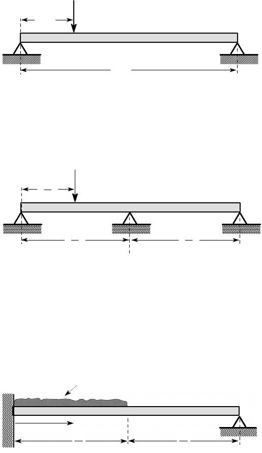
5.30. Figure P5.30 shows a beam on simple supports, loaded by a force F. Find the

value of F at plastic collapse if the fully plastic moment is M

Figure P5.30

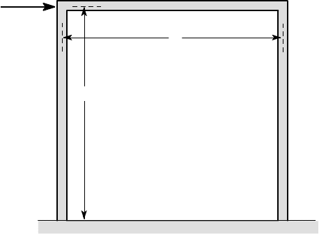
5.31. Figure P5.31 shows a beam on three simple supports subjected to a force F.

If the fully plastic moment for the beam is M

, ﬁnd the value of F that will cause

plastic collapse.

Figure P5.31

5.32*. Figure P5.32 shows a beam built in at one end, simply supported at the other

and loaded by a distributed load w

per unit length over one half of its length L.

Sketch the shape of the shear force and bending moment diagrams.

Show that a plastic hinge will form at some point z =d in the range 0 < d < L/2.

Determine d and the value of w

at collapse.

w per unit length

Figure P5.32

286 5 Non-linear and Elastic-Plastic Bending

5.33. The U-frame structure of Figure P5.33 is fabricated from three identical beams

of length L. It is built in at A,D and loaded by a horizontal force F at B. Find the

collapse load if the fully plastic moment for all segments of the beam is M

Figure P5.33

5.34. Re-solve Problem 5.33 if the supports at A,D are replaced by pin joints.

Shear and Torsion o f Thin-walled Beams

In Chapters 4 and 5, we investigated the stresses developed in beams subjected to

bending moments and, in some cases, an axial force — i.e. those forms of loading

that give rise to normal stresses

on transverse planes z= c, where c is a constant.

It is also worth noting that the combination of an axial force and a bending moment

is equivalent to an equal axial force with a different line of action (see for example

§5.5.2).

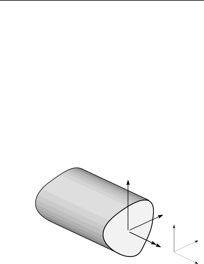
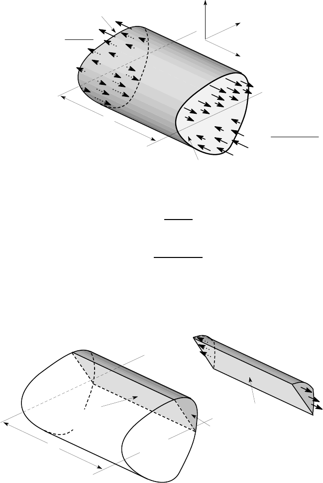
A similar relation exists between the two shear forces V

and the torque T ,

shown in Figure 6.1. All of these loads give rise to shear stresses on the transverse

plane A and in general the combination is statically equivalent to a resultant shear

force whose magnitude and direction is determined by V

, but whose line of action

is modiﬁed by the torque T .

Figure 6.1: Shear forces and torque on a transverse plane

The shear stress distribution due to the loading of Figure 6.1 can be obtained for

the elastic case, but the solution for general geometries is considerably more difﬁcult

than the bending theory and requires the solution of a partial differential equation

J.R. Barber, Intermediate Mechanics of Materials, Solid Mechanics and Its Applications 175,

2nd ed., DOI 10.1007/978-94-007-0295-0_6, © Springer Science+Business Media B.V. 2011

288 6 Shear and Torsion of Thin-walled Beams

with appropriate conditions at the boundaries of the section.

Fortunately, a more

straightforward approximate theory can be developed, which approaches the exact

theory in the important limiting case of thin-walled sections.

To introduce the subject, we shall ﬁrst revisit the derivation of the elementary

formula for the shear stress in a beam transmitting a shear force V . Later (in §6.3) we

shall draw on the ideas of §4.4.3 to extend the argument to a general unsymmetrical

section by choosing the coordinate system Oxy to coincide with the principal axes of

the section and using superposition.

6.1 Derivation of the shear stress formula

δz

M (z)

M (z + δz)

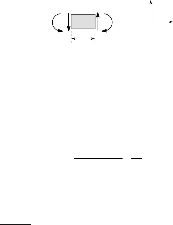
Figure 6.2: Equilibrium of a beam segment

Consider a small length

z of a beam, transmitting a shear force V

and a bending

moment M

as shown in Figure 6.2. As in Chapter 4, we deﬁne a coordinate system

such that the z-axis points along the beam and x,y are in the plane of the cross section.

The y-axis points upwards in Figure 6.2 and hence the x-axis must point into the

paper.

A positive moment M

is therefore clockwise on the positive z-surface, as

shown.

We assume that V

is constant along the beam, but M

cannot be constant, because

equilibrium of moments on the small element demands that

(z +

z) −M

(z) −V

z = 0

and hence

(z +

z) −M

(z)

. (6.1)

This well known result is of course widely used to ﬁnd the maximum bending

moment (where dM

/dz=0 and hence V

=0) and to sketch shear force and bending

moment diagrams, since the bending moment is the integral of the shear force and

hence is the area under the shear force diagram up to the point under consideration.

We next consider the bending stresses on the element of length

z shown in

Figure 6.3.

J.R.Barber (2010), Elasticity, Springer, Dordrecht, 3rd edn., Chapters 16,17.

Compare with Figure 6.1.

6.1 Derivation of the shear stress formula 289

neutral

axis

δz

M (z) y

σ =

M (z + δz) y

σ =

Figure 6.3: Bending stresses on the beam element

On the left end 1, we have

(z)y

, (6.2)

but on the right end 2,

(z +

z)y

. (6.3)

These stresses are statically equivalent to the moments in Figure 6.2 and hence the

element is in equilibrium as long as equation (6.1) is satisﬁed. However, if we make

a further cut longitudinally along the beam axis as shown in Figure 6.4 (a), the re-

sulting element [Figure 6.4 (b)] generally has different axial forces on its two ends

because of the differing values of

δz

longitudinal

cut

neutral

axis

longitudinal

cut surface

(a) (b)

Figure 6.4: (a) The longitudinal cut, (b) bending stresses on the section of the beam

element removed

290 6 Shear and Torsion of Thin-walled Beams

We shall refer to the area shaded in Figure 6.4 (a) as A

∗

to distinguish it from the

total area of the cross section A. Thus, A

∗

is the area of that part of the cross section

that is on one side of the longitudinal cut. The axial force on A

∗

at section 1 is

∗

dA =

(z)

∗

ydA , (6.4)

using (6.2). We recall from §4.3.1 that the integral in this equation, which is the ﬁrst

moment of the area A

∗

, can also be written A

∗

¯y

∗

where ¯y

∗

is the y-coordinate of the

centroid of A

∗

. Thus, we can rewrite (6.4) as

(z)A

∗

¯y

∗

. (6.5)

A similar argument for section 2 using equation (6.3) gives

(z +

z)A

∗

¯y

∗

. (6.6)

The forces F

and F

will not be equal unless A

∗

¯y

∗

= 0. If A

∗

were the whole

beam cross section, this condition would be satisﬁed by virtue of the choice of the

centroid of the section as coordinate centre, but it will not generally be satisﬁed

for that portion of the cross section removed by the longitudinal cut.

To keep the

element in equilibrium, there must therefore be an extra axial force and the only

place for this force to act is at the cut surface, since the axial forces on the transverse

sections have been taken into account already. This means there must be a horizontal

shear force Q=F

−F

on the cut, as shown in Figure 6.5. Thus

Q = F

−F

(z +

z) −M

(z)]A

∗

¯y

∗

¯y

∗

, (6.7)

using equation (6.1).

Figure 6.5: Equilibrium of the element of Figure 6.4(b)

The shear force per unit length of cut surface q, is obtained by dividing equation

(6.7) by

z, i.e.

q =

∗

¯y

∗

. (6.8)

In fact, it will be zero if and only if the centroid of A

∗

lies on the neutral axis.

6.1 Derivation of the shear stress formula 291

The quantity q is sometimes referred to as the shear ﬂow.

Up to this point, the above analysis is exact, within the limitations of the elemen-

tary beam theory, which itself can be shown to be exact as long as the shear force V

does not vary along the beam.

We can take a further approximate step if we assume

that the shear stress is uniform across the width t of the cut, in which case q=

t and

∗

¯y

∗

. (6.9)

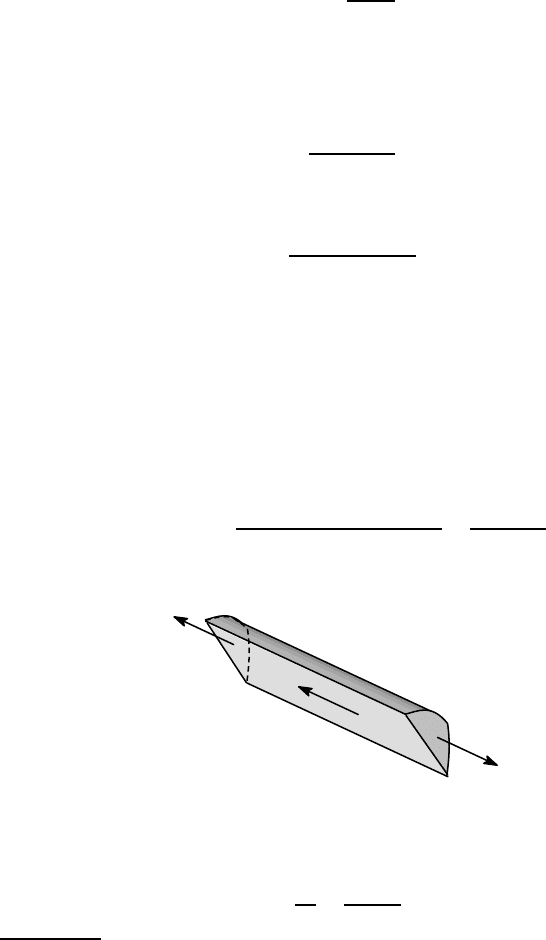
The stress calculated is a ‘longitudinal’ shear stress. It acts on the longitudinal

cut surface as shown in Figure 6.6 (a). Also,

is parallel with the beam axis, so it

points away from the cut line PQ at right angles. As discussed in §1.5.1, the stress

matrix (1.2) is symmetric and there must therefore be an equal complementary shear

stress pointing away from PQ on the end face, as shown in Figure 6.6 (b).

δz

(a) (b)

Figure 6.6: (a) Longitudinal shear stress on the cut surface, (b) complementary shear

stress on the transverse section

Thus,

is also the component of transverse shear stress at the cut pointing perpen-

dicularly into the area A

∗

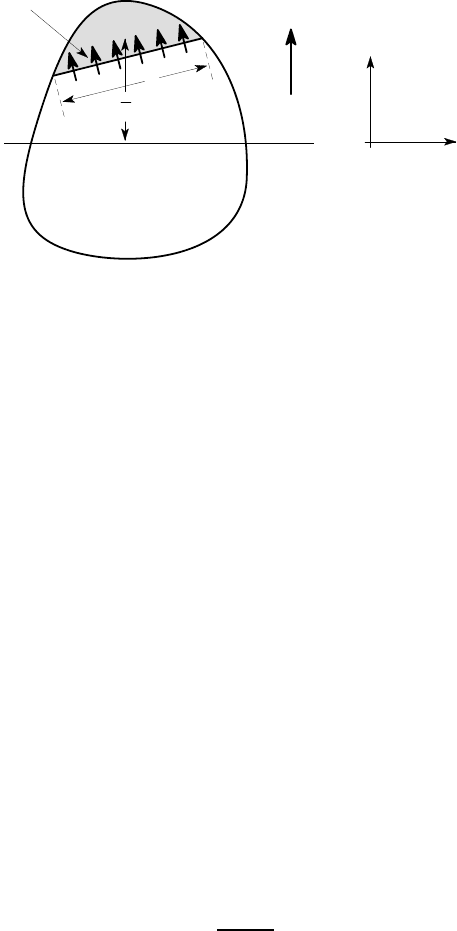
Summary

A common error is to misinterpret the quantities A

∗

, ¯y

∗

, t etc. appearing in the shear

stress equations (6.8, 6.9), so we here list their deﬁnitions for reference. These deﬁ-

nitions are illustrated in Figure 6.7.

∗

is the area of the transverse section removed by the longitudinal cut (shown

shaded in Figure 6.7).

¯y

∗

is the y-coordinate of the centroid of A

∗

measured from the neutral axis of bending

for the whole section.

t is the total length of the cut PQ. Notice that t appears in the formula because it

deﬁnes the width of the area available to transmit the longitudinal shear force Q.

Thus, if the cut passes through a hole in the section, only the segments through

the solid walls will contribute to t.

See, for example, J.R.Barber (2010), Elasticity, Springer, Dordrecht, 3rd edn., Chapter 17.

292 6 Shear and Torsion of Thin-walled Beams

is the shear force in the y-direction.

is the centroidal second moment of area of the whole section about the x-axis.

is the component of transverse shear stress at the line of the cut in the direction

pointing perpendicularly into the area A

∗

neutral

axis

Figure 6.7: Illustration of the deﬁnitions of A

∗

, ¯y

∗

,t,V

in equation (6.9).

We also note here that the product A

∗

¯y

∗

is the ﬁrst moment of the area A

∗

and it

is often conveniently obtained by splitting A

∗

into several rectangular areas A

,...

and summing A

¯y

+ ... as in §4.3.1.

6.1.1 Choice of cut and direction of the shear stress

In elementary treatments, the longitudinal cut is often taken to be parallel to the

neutral axis of bending, but no part of the preceding argument depends upon this

assumption. The results therefore apply for an arbitrary cut, which need not even

be a plane. The only requirement is that it should separate the original beam cross

section into two parts, one of which is identiﬁed as A

∗

It may require some explanation that the transverse shear stress on the end face

has components, i.e. it has magnitude and direction. A shear stress by deﬁnition has

to be parallel to the plane on which it acts, but in three dimensions, this still leaves

it two orthogonal directions in which to have components. By taking different cuts

through a given point, we can estimate both components of transverse shear stress,

but remember that we have made the assumption that

is uniform across t, so the

results may not be very accurate, particularly if we have reason to believe that the

distribution will be very non-uniform.

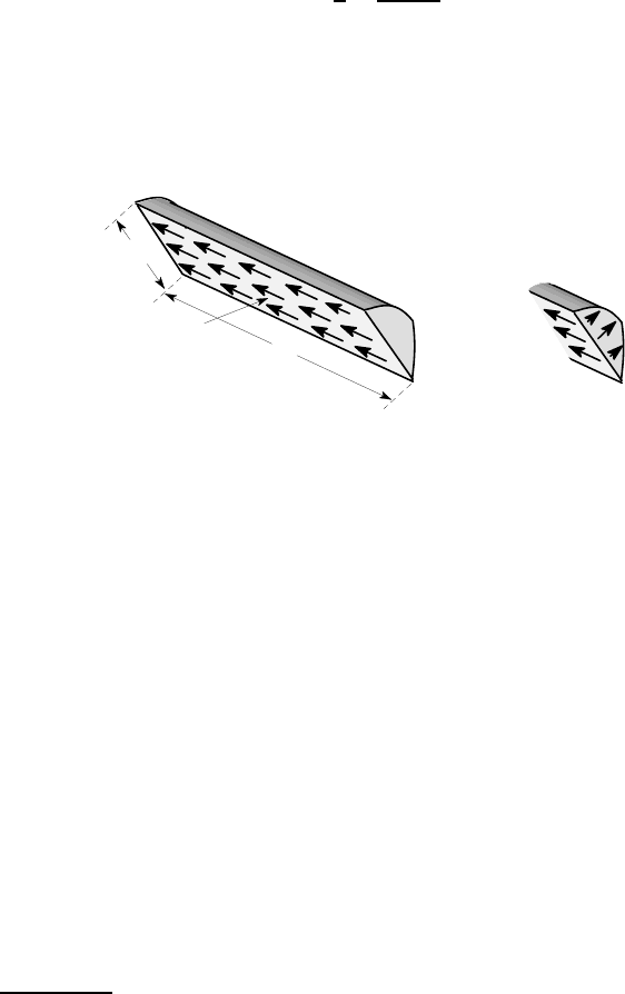
The most striking application of these arguments is in thin-walled open sections

such as the I-beam. With the cut BC in Figure 6.8 (a), A

∗

¯y

∗

is large, t is small and we

get a substantial vertical shear stress, as we should expect. However, if we make a

parallel cut DE in the ﬂange, as in Figure 6.8 (b), A

∗

¯y

∗

may still be fairly large, but

t is now also large, so

∗

¯y

∗

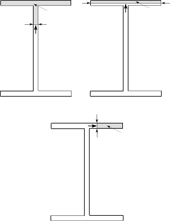
6.1 Derivation of the shear stress formula 293

will be small.

By contrast, if we make the cut FG through the ﬂange as in Figure 6.8 (c), A

∗

¯y

∗

will still be fairly large and t is now small, so that a signiﬁcant shear stress is ob-

tained. This stress has to point at the cut FG from the rest of the section and is

therefore a horizontal shear stress as shown in Figure 6.8 (c). Thus we conclude that,

in the ﬂange, the horizontal component of shear stress will be substantial, but the

vertical component will be small, giving a resultant that is predominantly horizontal.

B C

(a) (b)

(c)

Figure 6.8: Various cuts for the I-beam: (a) through the web, (b) horizontally through

the ﬂange, (c) vertically through the ﬂange

In general, when we have a thin-walled section, the shear stress component par-

allel to the wall will be signiﬁcant because the corresponding value of t is small,

294 6 Shear and Torsion of Thin-walled Beams

whereas that perpendicular to the wall will be negligible, because the corresponding

t is relatively large. In other words, the resultant shear stress tends to run parallel to

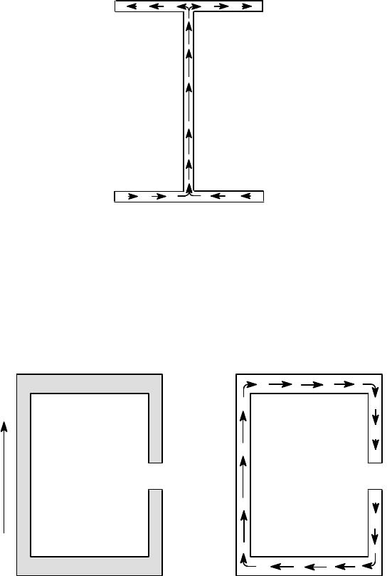
the thin walls of the section. In the I-beam, this results in the distribution shown in

Figure 6.9. This picture gives some idea of why q is referred to as the shear ﬂow,

since the shear stresses appear to ﬂow around the section like a ﬂuid. However, no-

tice that q is not generally constant — it is a maximum at the neutral axis, where

∗

¯y

∗

is maximum, and tends to zero at the ends of the section — i.e. at the ends of

the ﬂanges in the I-beam of Figure 6.9.

Figure 6.9: Shear stress distribution in the I-beam

Another unexpected result is obtained when the section bends back towards the

neutral axis, as in Figure 6.10 (a). In this case, the preceding arguments lead to the

stress distribution of Figure 6.10 (b) in which the shear stress near the ends acts

downwards on the section, despite the fact that the resultant is an upward shear force.

Notice however that the regions with downward shear stress have lower stress values,

being near to the free end (where the stress is always zero), so the resultant is an

upward force.

(a) (b)

Figure 6.10: Shear stress distribution for a slit rectangular tube