Battarbee R.W., Binney H.A. (Eds.) Natural Climate Variability and Global Warming: A Holocene Perspective

Подождите немного. Документ загружается.

100

Michel Cruciﬁx

Inductive and deductive climate models

It has become customary to deﬁne three categories of global climate models

(Claussen et al. 2002; Renssen et al. 2004) (Figure 4.2).

•

Conceptual models are made of a small number of differential equations designed

to represent interactions between the major climate components. They are called

inductive because the number of adjustable parameters is of the same order of mag-

nitude as the number of differential equations (number of degrees of freedom).

Their primary purpose is to formulate a phenomenological theory of climate

dynamics. This may cover problems as various as the stability of the ocean circula-

tion (Stommel 1961) or the astronomical theory of paleoclimates (Imbrie and

Imbrie 1980; Saltzman and Maasch 1990; Paillard 2001). Conceptual models can

produce very complex solutions that may even be chaotic. The conceptual models

that can successfully be tuned on the climate record provide a structure to observa-

tions which, according to information theory (Leung and North 1990), may confer

on them a prediction skill.*

•

Comprehensive climate models are built from ﬁrst principles of physics (equa-

tions of movement, radiative transfer, etc.) numerically implemented on three-

dimensional grids representing the atmosphere, the oceans, and sea-ice.† The

characteristic horizontal spatial scale of the grid is of the order of 100 km and the

* Saltzman (2002) considered as an “act of faith” that long-term climate dynamics may be described by

some low-order model, similar to thinking in physics that the cosmos is governed by a “uniﬁed

theory”. There is no easy demonstration of this, but Hargreaves and Annan (2002) showed that the

Saltzman and Maasch (1990) model does have signiﬁcant skill in predicting climate over about 100 kyr.

† Technically, the discretized equations of motion may be solved directly on the grid (grid-based mod-

els). Another possibility (spectral models) is to compute ﬁrst the spherical harmonics of the physical

quantities and then to resolve the equations of motion in this “conjugate” space. Differential operators,

such as the Laplacian, are indeed more easily expressed in the conjugate space. The spatial resolution of

a spectral model depends on the number of spherical transforms retained to perform the calculations.

For example, T32 means a triangular (T) truncation to the ﬁrst 32 spherical harmonics. This approxi-

mately corresponds to a resolution of 400 km × 400 km.

200 km

Millennium

Meso–

scale

models

DecadeYear

100 m

10 km

Day Century Milankovitch

20 km

100 km

Global

Continents/

oceans

Region

Regional

models

Comprehensive

models

EMICs

Inductive

models

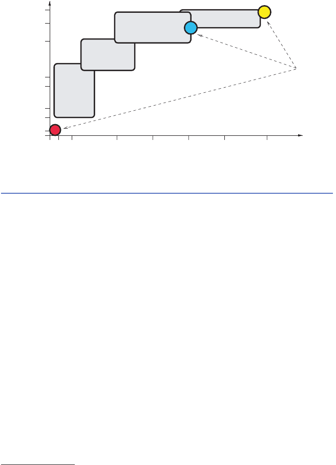
Figure 4.2 Time- and space-

scales covered by numerical

models used for weather and

climate prediction.

Conceptual models have only

a few degrees of freedom and

are designed to formulate and

test hypotheses in a very well-

deﬁned framework. Three

examples are given here: (1)

turbulence in the boundary

layer; (2) stability of the ocean

circulation; and (3) ice-sheet

response to astronomical

forcing. Comprehensive

climate models (also called

“general circulation models”)

include the largest number of

degrees of freedom and are

suitable to study climate

dynamics on time-scales of a

few decades to a few centuries.

Earth models of intermediate

complexity (EMICs) usually

cover longer time-scales.

Mesoscale and regional

models simulate weather and

climate over a limited domain

of the globe. A mesoscale

model typically covers a

domain the size of the UK,

and a regional model may

cover Europe or the USA.

9781405159050_4_004.qxd 6/3/08 3:54 PM Page 100

Modeling the climate of the Holocene

101

integration time step is a few hours (see Johns et al. (2006) for a recent example).

Synoptic atmospheric variability is thus explicitly calculated. Comprehensive

climate models are “deductive” because the number of constitutive equations is

several orders of magnitude larger than the number of adjustable parameters.

Phenomena occurring at spatial scales smaller than the model grid, such as convec-

tive cloud formation, are parameterized by means of phenomenological equations.

Climate modelers establish these equations on the basis of local observations

(soundings, aircraft measurements, surface data) and specialized models. A para-

meterization has to be “physically reasonable” and respect conservation principles

(conservation of energy, entropy, momentum, etc.). In spite of these constraints,

different mathematical formulations of a parameterization may seem to provide

equally good results and there is no easy way to know which one is best. This is what

is called structural uncertainty.

In practice, the parameters need to be tuned again so that the climate generated

by the global model agrees with observed global-scale features of the climate

system (e.g. the existence of a meridional overturning cell in the North Atlantic).

This tuning process is too often viewed as a necessary evil about which little detail is

given in the model documentation.

Fortunately, tuning tends to be better recognized as a natural step of model

development. Model parameters are attributed uncertainty ranges (constrained by

laboratory measurements and local observations), and the likelihood of a given

parameter combination is estimated from the agreement between the model and a

well-deﬁned set of global observations (surface temperature, precipitation, satel-

lite estimates of the radiative balance, etc.) (more detail is given below).

Nowadays, the development of comprehensive models mobilizes large multi-

disciplinary teams driven by the aim of providing reliable future climate predic-

tions. These models must therefore include all processes relevant at the decadal

to century time-scales with as much detail as computational power permits. This

covers various aspects such as soil dynamics, vegetation dynamics, ocean biogeo-

chemistry, ice-sheet dynamics, and river hydrology. At the time of writing, a

100-year long simulation of climate with a comprehensive climate model (e.g.

1.5 × 1.5° resolution) requires more than a month of a supercomputer with power-

ful data storage facilities.

•

Earth models of intermediate complexity (EMICs) ﬁll the gap between

conceptual and comprehensive climate models (Claussen et al. 2002). They resem-

ble comprehensive climate models but calculations are made on longer time-scales

and larger spatial scales. The degree of parameterization is higher, which may

imply a larger structural uncertainty. Yet, like comprehensive models, the number

of degrees of freedom in EMICs exceeds the number of adjustable parameters by

several orders of magnitude. The EMIC category covers a range of models that may

be used to study interdecadal to astronomical time-scales depending on the model.

Examples of EMICS used to study the Holocene are given in Table 4.1.

Earth models of intermediate complexity and conceptual models are useful

because they cover spatial and temporal scales for which comprehensive models

9781405159050_4_004.qxd 6/3/08 3:54 PM Page 101

102

Michel Cruciﬁx

are not suitable. Consider the glacial–interglacial cycles: the growth and decay of

the total continental ice mass at the glacial–interglacial time-scale is of the order of

a few centimeters of sea-level equivalent per year. These one or two centimeters

result from a difference between total evaporation, precipitation, melting, and

freezing that is so small compared with the quantities themselves that it cannot be

conﬁdently estimated by a general circulation model (Saltzman 1988, 2002). In

fact, the present net accumulation rates of snow over Antarctica and Greenland are

even not accurately known (Rignot and Thomas 2002). Earth models of interme-

diate complexity provide a solution. They may be tuned to reproduce reasonable

results over a given section of a glacial–interglacial cycle (e.g. the last glacial incep-

tion, as in Gallée et al. 2002) and then used to study other periods (Loutre et al.

2007).

We have so far considered global climate models. Comparison with (paleo) data

may make it necessary to resolve smaller spatial scales than those of a comprehen-

sive climate model. The method demanding least computing time is statistical

downscaling (Murphy 1998), where statistical relationships are applied between

climate variations at the synoptic scale (200–300 km) and the local climate. Two

more elaborate strategies are documented in the literature: nesting and zooming

(Giorgi and Mearns 1999). Under “nesting”, output of a global model is used to

drive a regional dynamical model of the atmosphere that resolves horizontal length

scales of the order of 30 to 50 km. “Regional” indicates that this high-resolution

model only covers a deﬁned region of the globe, such as Europe. Zooming is based

Table 4.1 Examples of Earth models of intermediate complexity (EMICs) used to study the Holocene

Model

LLN-2D

MoBidiC

CLIMBER-2

Green McGill

Paleoclimate Model

ECBILT (coupled to a

low-resolution ocean model)

ECBILT–CLIO (coupled to a higher

resolution ocean–sea-ice model)

Reference

Loutre et al. 2007

Cruciﬁx et al. 2002

Bauer et al. 2004

Ganopolski et al. 1998

Claussen et al. 1999;

Claussen et al. this volume

Brovkin et al. 2002

Wang et al. 2005a

Wang et al. 2005b

Wang and Mysak 2005

Weber and Oerlemans 2003

Renssen et al. 2005

Renssen et al. 2002

Example of published applications over the Holocene

Prediction of the next glacial inception

Vegetation–climate interactions at high latitudes

Impact of freshwater input in the North Atlantic around 8000 years ago

Factor decomposition (see text)

Desertiﬁcation of the Sahara in response to orbital forcing

Changes in ocean and terrestrial carbon storages during the Holocene

Analysis of the carbon budget

Existence of a climate optimum after the disappearance of the

Laurentide Ice Sheet

Impact of freshwater input in the North Atlantic around 8000 years ago

The inﬂuence of changes in precipitation and temperature on the

evolution of three representative glaciers

See text

Impact of freshwater input in the North Atlantic around 8000 years ago

9781405159050_4_004.qxd 6/3/08 3:54 PM Page 102

Modeling the climate of the Holocene

103

on a comprehensive climate model featuring an irregular mesh reﬁned over the

region of interest in order to capture the smaller spatial scales.

Initial conditions, boundary conditions, and

model parameters

Mathematically speaking, a climate model is a system of equations with diagnostic

and prognostic equations. Diagnostic equations instantaneously link different

variables to each other, for example, the hydrostatic assumption linking pressure

and density. Prognostic equations need to be integrated forward in time, for exam-

ple, the Navier–Stokes equations describing hydrodynamics. In theory, it should

be possible to integrate prognostic equations backwards in time, but this task is

almost insurmountable because many diagnostic relationships are nonbijective

(i.e. cannot easily be inverted). The model is thus integrated forward in time and

one must deﬁne initial conditions, boundary conditions, and parameters.

•

Initial conditions represent the climate state from which the model equations

are integrated. They are generally supplied from a previous experiment or from

observations.

•

Boundary conditions deﬁne values or ﬂuxes at the boundary of the domain, such

as the surface topography and incoming shortwave radiation at the top of the

atmosphere. The latter is calculated from the geometry of the Earth’s orbit.

•

Parameters are constants used in the equations. Some are directly speciﬁed from

laboratory experiments (e.g. heat capacity of water) or direct observations (albedo

of sea-ice, concentrations of greenhouse gases). Others are more phenomenological

and they must be calibrated by comparing model results with observations (see below).

Once initial conditions, boundary conditions, and parameters are speciﬁed, the model

is run to perform either an steady-state experiment or a transient experiment.

The climate modeler’s “steady-state experiment” is an integration for which

boundary conditions and parameters are constant, except for the insolation

seasonal cycle. Such experiments are suited to study the statistics of a quasi-steady

climate, where the time-scale of the external forcing change is larger than the

longest dissipative time-scale of the system. This is about a few thousand years if

deep-ocean dynamics are taken into account (this number is reached by dividing

the depth of the ocean to the square by the turbulent vertical diffusion coefﬁcient).

Initial conditions seem unimportant in steady-state experiments because they are

eventually dissipated (“forgotten”). There are two caveats to this statement. First,

it is more economical to guess initial conditions that are not too far from the

solution in order to reduce as much as possible the time spent by the system to

reach it (spin-up time). Second, there may be two quasi-state solutions to the

model equations, with only a small probability of transition from the one to

the next: For example, a green and a white Sahara (Claussen, this volume). An

experiment is said to be transient if the boundary conditions and some other

9781405159050_4_004.qxd 6/3/08 3:54 PM Page 103

104

Michel Cruciﬁx

parameters (such as greenhouse gas concentrations) change during the integra-

tion. These changes constitute an external forcing that inﬂuences the climate

trajectory. Two categories of transient experiments may be distinguished. In the

ﬁrst one, the external forcing varies slowly or at a rate comparable to the dissipative

time-scales of the system. A good example is the change in the spatial and seasonal

incoming solar radiation due to the quasi-cyclic variations in the Earth’s orbit:

eccentricity, precession, and tilt of the rotation axis on the ecliptic (i.e. orbital

forcing). Such experiments allow us to identify and understand nonlinear pro-

cesses in the response to the forcing, such as deglaciation or desertiﬁcation of the

Sahara (Claussen et al. 1999). The response is said to be abrupt if its characteristic

time-scale is shorter than that of the forcing (Alley et al. 2003). The second

category of transient experiments gathers those in which the forcing varies with a

characteristic time shorter than the dissipative time-scales of the system. In this

case the abrupt character of the response is due to the forcing itself. Experiments

of this kind are usually performed to test hypothetical scenarios such as a discharge

of freshwater in the ocean (Renssen et al. 2001; Bauer et al. 2004; LeGrande

et al. 2006).

Model–data comparison versus data assimilation

The classic methodology assumes a clear distinction between model input (initial

conditions, boundary conditions, parameters) and output (the predicted climate).

Boundary conditions and parameters are considered as “known” and there is no

formal uncertainty attached to them. The model output is then compared with

observations. There is usually a pair of experiments. One is designed to produce

a simulation of the pre-industrial climate and, in the other, boundary conditions

and certain parameters (such as greenhouse gas concentrations) are modiﬁed to

predict past climate.

The Paleoclimate Modeling Intercomparison Project (PMIP) framed past

climate simulations (mid-Holocene and Last Glacial Maximum) with different

comprehensive climate models and organized a systematic comparison between

the model output and paleoclimatic data (Joussaume and Taylor 2000; Braconnot

et al. 2007) (Figure 4.3). Appropriate proxy models may facilitate the model–data

comparison. Proxy models are calibrated to map climate model outputs on observ-

able quantities such as the dominant biome (Haxeltine and Prentice 1996), lake

level, or glacier length (Weber and Oerlemans 2003). Climate models may also

directly include the necessary equations to simulate observable features such as

dust ﬂux (Joussaume and Jouzel 1993a), oxygen (Joussaume and Jouzel 1993b),

carbon (Marchal et al. 1999), and boron isotopic ratios (LeGrande et al. 2006).

It was shown that climate models correctly reproduce a number of observed

features of the mid-Holocene climate: increased precipitation in the Sahel,

decreased precipitation in South America, reduced sea-ice cover in the Norwegian

Sea, northward advance of boreal forest in Russia, and reduced frequency of El

9781405159050_4_004.qxd 6/3/08 3:54 PM Page 104

Modeling the climate of the Holocene

105

....

–4

–3

–2

–1

–0.5

–0.25

0.25

0.5

0 180E90E180W

90W

90N

45S

45N

90S

–1

–0.5

-0.25

–0.25

-0.25

–0.25

0.25

0.5

0 180E90E180W 90W

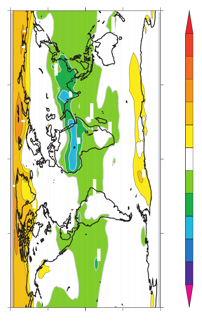
Figure 4.3 Change in annual mean surface temperature induced by switching from today’s orbital forcing to that of 6000 years ago (see also Figure 4.4) as

simulated by Paleoclimate Modeling Intercomparison Project (PMIP) models (the mean model response is displayed). The plot evidences well the annual

polar warming and equatorial cooling. Sensitivity experiments suggest that the annual tropical cooling is mainly caused by the increase in obliquity and the

resulting decrease in annual mean insolation below 43° of latitude. The polar warming results from a combination of obliquity (larger annual mean

insolation, concentrated in summer) and precession (larger summer and autumn insolation). Seasonal changes in insolation are translated into an annual

temperature signal by the sea-ice feedback. Cooling of northern sub-tropical deserts is a signature of enhanced summer monsoon precipitation and the

resulting increase in surface evaporation. Note that the vegetation response was not taken into account in these experiments. (Data were supplied by

Jean-Yves Peterschmitt and extracted from the PMIP database in Saclay, France.)

9781405159050_4_004.qxd 6/3/08 3:54 PM Page 105

106

Michel Cruciﬁx

Niño events (see the recent reviews by Braconnot et al. 2004; Renssen et al. 2004;

Cane et al. 2006; pioneering work is covered in Wright et al. 1993). It is then pos-

sible to decrypt the mechanisms of these climate changes by means of appropriate

sensitivity experiments. One method, known as “factor separation” (Stein and

Alpert 1993), consists in sequentially freezing certain components such as vegeta-

tion or sea-ice distribution normally calculated by the model. It was used by

Ganopolski et al. (1998) to show that hemispheric warming in response to mid-

Holocene orbital parameters results from feedbacks between boreal vegetation and

sea-ice (in the CLIMBER model) (see also Harvey 1988; Cruciﬁx and Loutre 2002).

More generally, feedback analysis of mid-Holocene experiments has highlighted

the importance of ocean dynamics and vegetation and justiﬁed including vegeta-

tion dynamics in climate models used for future climate prediction.

Climate models are never in “perfect agreement” with data. For example, the

“IPSL” (i.e. the climate model of the “Institut Pierre et Simon Laplace” in Saclay,

France) model simulation of the mid-Holocene climate indicates, compared with

the present-day, increased aridity in central Eurasia and a northward advance of

the boreal forest’s northern limit in Canada, contrary to observations (Wohlfahrt

et al. 2004). Climate modelers tend to be very defensive when it comes to

model–data comparisons because discrepancies call the model performance into

question. This attitude is unfortunate because model–data differences contain

particularly useful information. There are at least two things the modeler would

like to know about them. First, what is their cause? Are they due to a process badly

accounted for, an inadequate boundary condition (e.g. incorrect speciﬁcation of

ice sheets) or a data misinterpretation? Second, does this disagreement affect the

model’s prediction of future climate change?

A new methodology is being formalized to address these questions, called “prob-

abilistic inference with climate models” or “climate data assimilation” (Rougier

2006). The fundamental idea is to attribute explicitly uncertainty ranges to model para-

meters, which are explored by performing large ensembles of sensitivity experi-

ments. A likelihood is attributed to a parameter value depending on (i) the difference

between the model prediction obtained with this parameter value and the data-

estimate, (ii) the data uncertainty, and (iii) prior knowledge on the parameter.

This is a data assimilation because observations (temperature, precipitation, etc.)

provide explicit constraints on model parameters and/or boundary conditions.

Climate data assimilation may help us to reﬁne estimates on phenomenological

parameters used in parameterizations. It therefore provides a formal framework to

“tuning” by clarifying which information is being used to constrain parameters

and estimate probability distribution functions on both model input and output.

The trouble with this process is that it puts a high demand on computing

resources because it requires numerous experiments. It has therefore been imple-

mented in only a few cases using modern climatic observations (Murphy et al.

2004), plus a small number of studies using large-scale estimates of the Last Glacial

Maximum temperature (Annan et al. 2005; Schneider von Deimling et al. 2006).

Examples above are based on steady-state experiments. Data assimilation also

applies to transient experiments. In short experiments (i.e., time length shorter

9781405159050_4_004.qxd 6/3/08 3:54 PM Page 106

Modeling the climate of the Holocene

107

than the dissipative time-scales of the system), data assimilation is used to provide

estimates of climate variables for which there is no direct observation (e.g. Goosse

et al. this volume) by constraining initial conditions (cf. Jones and Widdmann

2004; van der Schrier and Barkmeijer 2005). In long transient simulations, data

assimilation may be used to constrain model parameters (Hargreaves and Annan

2002) (see below).

How long will the Holocene last?

The Holocene is a particularly long episode of stable climatic conditions compared

with the three previous interglacial periods (Sirocko et al. 2007). Its stability

certainly favored the establishment of modern civilizations. What explains the

stability of the Holocene, and how long will it be?

Modeling the long-term evolution of climate requires taking into account

changes in the spatial and seasonal distribution of incoming shortwave radiation

(insolation) at the top of the atmosphere (Figure 4.4). The latter is fully deter-

mined by three parameters: eccentricity, obliquity, and climatic precession (Berger

1978). Eccentricity is a geometric measure of the stretching of the Earth’s orbit.

It varies between about 0.002 and 0.040 on periods of 400 000 and 100 000 years.

It is presently small (0.016) and a minimum will be reached in 27 000 years.

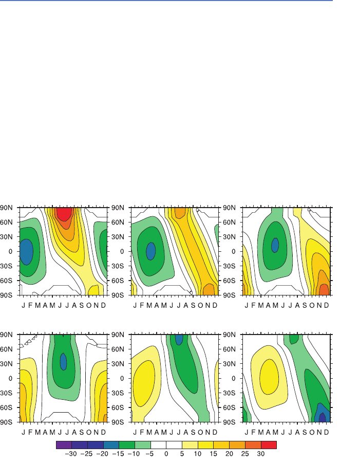
Insolation anomaly (W m

–2

)

9 kyr BP 6 kyr BP 3 kyr BP

3 kyr AP

6 kyr AP

Present

Figure 4.4 Month–latitude

distribution of incoming

shortwave radiation

(insolation) received from the

Sun at the top of the

atmosphere between 9000

years BP and 6000 years AP

(after present). A mean

distribution assuming no

eccentricity and a mean

obliquity of 23°20′ was

subtracted in order to

highlight the effects of

precession and obliquity

changes. Precession

redistributes heat across the

seasons (positive anomaly

around July 9000 years BP

and positive anomaly around

January at present). The

decrease in obliquity during

the Holocene contributes to

reduce summer insolation in

both hemispheres.

9781405159050_4_004.qxd 6/3/08 3:54 PM Page 107

108

Michel Cruciﬁx

Obliquity is the angle between the Equator and the orbital plane (ecliptic). It varies

between 22 and 25° with a period of 40 000 years. Obliquity has decreased by 0.8°

during the past 9000 years, and it will continue to decrease over the next 10 000

years. As a consequence, the distribution of insolation is being slightly modiﬁed

with (i) less insolation available to the summer hemisphere, with highest differ-

ences at high latitudes, and (ii) a decrease in annual mean insolation polewards of

43°N and 43°S, symmetric about the Equator, which compensates for a corres-

ponding increase equatorwards of 43°. Changes in annual mean insolation are

small (1 to 2 W m

−2

) but provisional calculations conﬁrmed by sensitivity experi-

ments with a comprehensive climate model reveal that the corresponding thermal

forcing easily explains sea-surface temperature changes by 0.5 to 1°C (Liu et al.

2002; Loutre et al. 2004). Precession is the cycling of the angle formed by the posi-

tion of the Earth on 21 March, the Sun, and the point of the orbit closest to the

Sun (perihelion). The cycle takes about 21 000 years. Perihelion was reached in July

11 000 years ago. It then drifted from July to later in the year. It occurs in January

today. Given that insolation decreases with the square of the Earth–Sun distance,

precession during the Holocene caused a decrease in June insolation and a corre-

sponding increase in January. Precession does not alter annual mean insolation at

any latitude. The seasonal redistributing action of precession makes it an efﬁcient

modulator of seasonal weather systems, such as tropical monsoons (Kutzbach and

Otto-Bliesner 1982; Harrison et al. 2003; Braconnot et al. 2004). These effects

naturally become less important when eccentricity decreases as at present.

All comprehensive model experiments so far have demonstrated that orbital

forcing induces signiﬁcant and measurable changes in temperature, precipitation,

and atmospheric circulation. These changes constitute the “fast” climate response

to orbital forcing, which drives – and may be altered by – the slow components of

the climate system (ice sheets, deep-ocean dynamics, ocean biogeochemistry,

vegetation) over several millennia.

Conceptual models provide a convenient theoretical framework to study free

and forced interactions between the slow components of the climate system. A par-

ticularly signiﬁcant development is Saltzman’s model of the Late Cenozoic Ice

Ages (Saltzman and Maasch 1990). This three-equation model with nine para-

meters represents the interactions between the carbon cycle, ice sheets, and ocean

circulation. Probabilistic inference with this model (Hargreaves and Annan 2002)

indicates an immediate end to the Holocene, with ice volume reaching a maximum

in around 60 kyr (assuming no anthropogenic perturbation). But is this prediction

correct? For example, it is noted that the Saltzman–Maasch model fails to repro-

duce the steadily increasing trend in CO

concentration during marine isotope

stage (MIS) 11 (after termination V, 400 000 years ago) (Raynaud et al. 2005;

Siegenthaler et al. 2005). Therefore, some stabilizing mechanisms may have been

ignored in this model. We therefore turn to another conceptual model presented

by Paillard (2001).

Paillard’s conceptual model features three possible climate regimes (glacial,

mild glacial, interglacial) to which the system is successively attracted depending

on insolation and ice volume. Contrary to Saltzman’s, Paillard’s model succeeds in

9781405159050_4_004.qxd 6/3/08 3:54 PM Page 108

Modeling the climate of the Holocene

109

predicting the correct length for MIS 11 (two precession cycles). Paillard’s model

can then be used to predict the length of the Holocene. The result is ambiguous.

The prediction can either be a short Holocene (glacial inception already begun) or

a very long one (glacial inception in 50 kyr) depending on the model parameters.

Yet the tested parameter values seem equally reasonable: the model provides a

satisfactory ﬁt to data of the past 800 kyr (Imbrie et al. 1984) in both cases. Only the

observation that we are presently not undergoing a glaciation allows us to reject

the ﬁrst solution. In other words, the length of the Holocene would not have been

predictable 9000 years ago with Paillard’s model.

There is presently no comprehensive model or even an EMIC (see above) cap-

able of representing the interactions between the slow components of the climate

system satisfactorily enough to predict the evolution of ice volume and greenhouse

gas concentrations over several glacial–interglacial cycles. There are a few EMICs,

however, that are able to simulate the evolution of the atmosphere–ocean–ice-sheet

system on those time-scales: the LLN-2D model (Gallée et al. 1991, 1992),

CLIMBER-2 (Petoukhov et al. 2000; Calov et al. 2005), and the Toronto climate–

ice-sheet model (Tarasov and Peltier 1999). The LLN-2D model is particularly suit-

able to study the evolution of ice volume in response to hypothetical CO

scenarios

and orbital forcing because it successfully reproduces several past glacial–interglacial

cycles assuming that the evolution of greenhouse gas concentrations is correctly

prescribed (Loutre and Berger 2003).

Both CLIMBER and LLN-2D consistently show no glacial inception during the

Holocene when observed CO

concentrations are prescribed (Claussen et al. 2005;

Loutre et al. 2007). Other CO

scenarios were then tested. Neither LLN-2D nor

CLIMBER predicted a modern glacial inception as long as CO

remained above

240 ppmv during the Holocene. The LLN-2D further shows that even if CO

con-

centration decreased in the future down to glacial levels, glaciation will not occur

before 50 000 years (Loutre et al. 2007).

The quasi-absence of precessional forcing due to the weak eccentricity may

therefore explain the exceptional stability of the Holocene. This statement, how-

ever, calls for a few clariﬁcations. First, sensitivity experiments with the LLN-2D

model suggest that there is actually a window, roughly between −5000 and +5000

years from now, during which a low enough CO

concentration (below 240 ppmv)

induces a glacial inception (Figure 4.5, red line). This is consistent with sensitivity

experiments with a more comprehensive model calibrated on the present-day

climate showing accumulation of perennial snow for 240 ppmv CO

and 450 ppbv

(Ruddiman et al. 2005) (the methane feedback is implicitly taken into account

in the LLN-2D via the model calibration on previous glacial–interglacial cycles).

These results conﬁrm Paillard’s prediction that the present orbital conﬁguration

may be compatible with a glacial inception (Paillard 2001), but they also show that

the inception scenario is no longer possible given the present CO

concentration.

Second, the LLN-2D predicts a three-precession cycle duration for MIS 11 when

forced by the Vostok CO

concentrations (Petit et al. 1999), but sensitivity experi-

ments with slightly lower CO

concentrations result in a short MIS 11 (Loutre and

Berger 2003). Paillard (2001) also found that small parameter changes may make

9781405159050_4_004.qxd 6/3/08 3:54 PM Page 109