Bhushan B. Handbook of Micro/Nano Tribology, Second Edition

Подождите немного. Документ загружается.

found that the surface heights of a ground-glass surface were not symmetric like the normal distribution

but were best ﬁtted by an ICS distribution with ν = 21.

4.3.2 RMS* Values and Scale Dependence

A rough surface is often assumed to be a statistically stationary random process

(Papoulis, 1965). This

means that the measured roughness sample is a true statistical representation of the entire rough surface.

Therefore, the probability distribution and the standard deviation of the measured roughness should

remain unchanged, except for ﬂuctuations, if the sample size or the location on the surface is altered.

The properties derived from the distribution and the standard deviation are therefore unique to the

surface, thus justifying the use of such roughness characterization techniques.

Because of simplicity in calculation and its physical meaning as a reference height scale for a rough

surface, the rms height of the surface is used extensively in tribology. However, it was shown by Sayles

and Thomas (1978) that the variance of the height distribution is a function of the sample length and

in fact suggested that the variance varied as

(4.3.6)

where L is the length of the sample. This behavior implies that any length of the surface cannot fully

represent the surface in a statistical sense. This proposition was based on the fact that beyond a certain

length, L, the surface heights of the same surface were uncorrelated such that the sum of the variances

of two regions of lengths L

and L

can be added up as

(4.3.7)

They gathered roughness measurements of a wide range of surfaces to show that the surfaces follow the

nonstationary behavior of Equation 4.3.6. However, Berry and Hannay (1978) suggested that the variance

can be represented in a more general way as follows:

(4.3.8)

where n varies between 0 and 2.

If the exponent n in Equation 4.3.8 is not equal to zero of a particular surface, then the standard

deviation or the rms height, σ, is scale dependent, thus making a rough surface a nonstationary random

process. This basically arises from the multiscale structure of surface roughness where the probability

distribution of a small region of the surface may be different from that of the larger surface region as

depicted in Figure 4.4b. If the larger segment follows the normal distribution, then the magniﬁed region

may or may not follow the same distribution. Even if it does follow the normal distribution, the rms σ

can still be different.

Other statistical parameters that are also used in tribology (Nayak, 1971, 1973) are the rms slope, σ′

and rms curvature, σ″

, deﬁned as

(4.3.9)

*The rms values (of height, slope, or curvature) are related to the corresponding standard deviation, σ, of a surface

in the following way: rms

= σ

+ z

, where z

is the mean value. In this chapter it will be assumed that z

= 0; that

is, the mean is taken as the reference, such that rms = σ.

≈ L

σσσ

LL L L+

()

≈ L

′

∂

()

∂













−

()

−

()













∫

∑

−

ij ij

zx y

zx y zx y

,,,

∆

(4.3.10)

Here, although the rms slope and the rms curvature are expressed only for the x-direction, these values

can similarly be obtained for the y-direction. These parameters are extensively used in contact mechanics

(McCool, 1986) of rough surfaces.

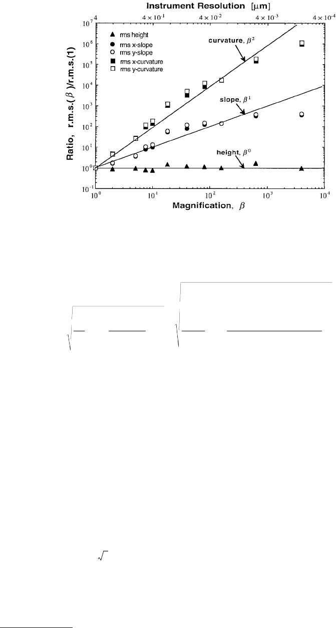
The question that now remains to be answered is whether the rms parameters σ, σ′, and σ″ vary with

the statistical sample size or the instrument resolution. Figure 4.6 shows the rms data for a magnetic tape

surface (Bhushan et al., 1988; Majumdar et al., 1991). Along the ordinate is plotted the ratio of the rms

value at a magniﬁcation, β, to the rms value at magniﬁcation of unity. The magniﬁcation β = 1 corre-

sponds to an instrument resolution of 4 µm and scan size of 1024 × 1024 µm containing 256 × 256

roughness data points. The roughness data in the range 1 < β < 10 were obtained by optical interferometry

(Bhushan et al., 1988), whereas for β > 10, the data were obtained by atomic force microscopy (Majumdar

et al., 1991; Oden et al., 1992). An increase in β corresponds to an increase in instrument resolution with

the highest being equal to 1 nm. The data clearly show that the rms height does not change over ﬁve

decades of length scales and can therefore be considered scale independent over this range of length scales.

However, the rms slope increases with magniﬁcation as β

and the rms curvature increases as β

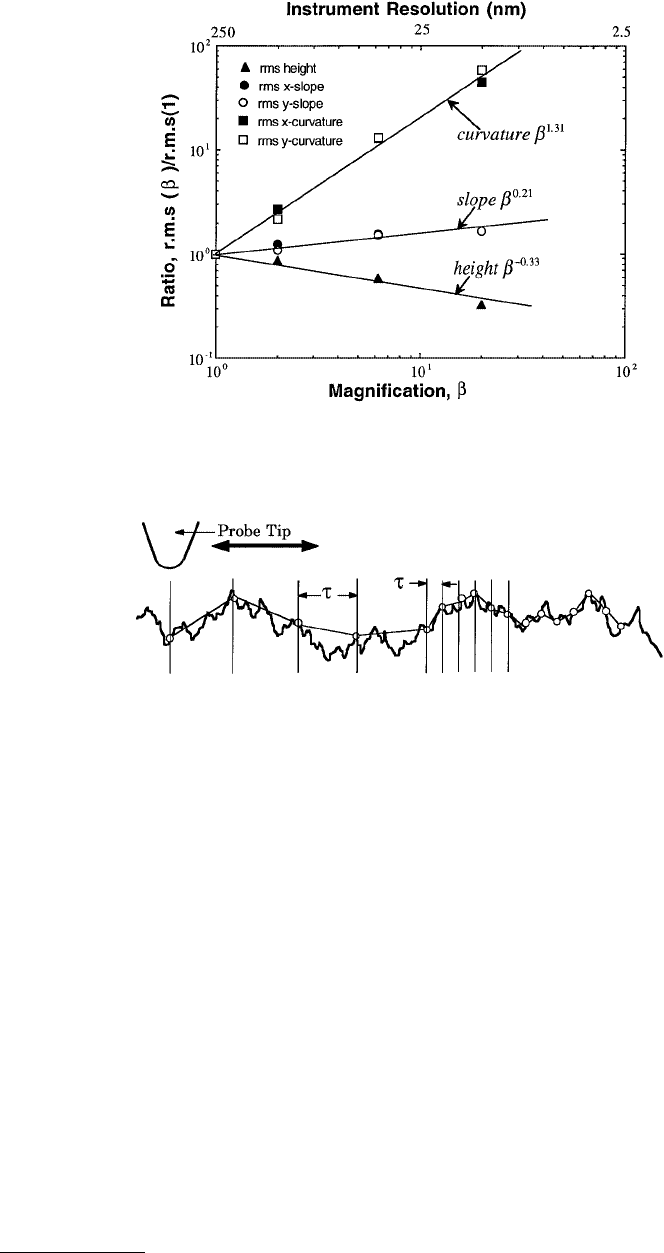
. Figure 4.7

shows similar variations for a polished aluminum nitride surface where the roughness data was obtained

by atomic force microscopy. In this case, the rms height σ reduces with decreasing sample size but does

not follow the trend σ ≈ as suggested by Sayles and Thomas

(1978). Nevertheless, the variation does

make the surface a nonstationary random process. The rms slope and the rms curvature, on the other

hand, increase with the instrument resolution, as observed in Figure 4.7.

Although Figures 4.6 and 4.7 show statistics for speciﬁc surfaces, the trends are typical for most rough

surfaces that have been examined. The following can be concluded from these trends. The rms height,

FIGURE 4.6 Variation of rms height, slope, and curvature of a magnetic tape surface as a function of magniﬁcation,

β, or instrument resolution. The vertical axis is the ratio of an rms quantity at a magniﬁcation β to the rms quantity

at magniﬁcation of unit, which corresponds to an instrument resolution of 4 µm. Roughness measurements of β <

10 were obtained by optical interferometry (Bhushan et al., 1988), whereas that for β > 10 were obtained by atomic

force microscopy (Oden et al., 1992).

′′

∂

()

∂













−

()

−

()













∫

∑

−

ij ij

zx y

zx y zx y

zx y

∆

σ, is a parameter which could be scale independent for some surfaces but is not necessarily so for other

surfaces. The rms slope, σ′, and the rms curvature, σ″, on the other hand, always tend to be scale

dependent. Therefore, the rms height can be used to characterize a rough surface uniquely if it is scale

independent, as is the case of the magnetic tape surface in Figure 4.6. However, it is not clear under what

conditions the rms height is scale dependent or independent. These conditions will be explored in the

Section 4.3.3. However, the reasons can be qualitatively shown by the self-repeating nature of the surface

roughness depicted in Figure 4.8.

Given a rough surface, an instrument with resolution τ will measure the surface height of points that

are separated by a distance τ. If τ is reduced, new locations on the surface are accessed. Due to the multiple

scales of roughness present, a reduction in τ makes the measured proﬁle look different for the same

surface. When τ is reduced, it is found that the straight line joining two neighboring points becomes

steeper on an average, as qualitatively observed in Figure 4.8. This increases the average slope and the

curvature of the surface. Therefore, the slope and the curvature fall victim to the “rough or smooth”

dilemma that is qualitatively discussed in Section 4.2. Figures 4.6 and 4.7 quantitatively exhibit scale

dependence of the rms slope and curvature. One can conclude these parameters cannot be used to

characterize a rough surface uniquely since they are scale dependent; that is, the use of these parameters

in any statistical theory of tribology can lead to erroneous results. It is thus necessary to obtain some

scale-independent techniques for roughness characterization.

FIGURE 4.7 Variation of rms height, slope, and curvature of a polished aluminum nitride surface as a function of

magniﬁcation, β, or instrument resolution.

FIGURE 4.8 Illustration of roughness measurements at different instrument resolution τ. As τ is reduced, the

surface that is measured is quite different, as qualitatively shown. The average slope and the average curvature of the

proﬁle is higher for smaller τ.

4.3.3 Fractal Techniques

4.3.3.1 A Primer for Fractals

The self-repeating nature of surface roughness has not only been found in surfaces but also in several

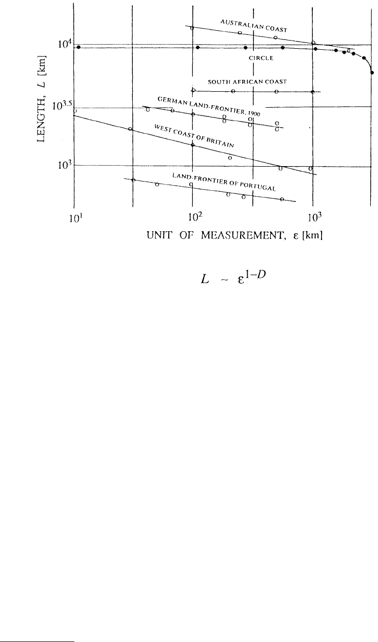
objects found in nature. In his classic paper, Mandelbrot (1967) showed that the coastline of Britain has

self-similar features such that the more the coastline is magniﬁed, the more features and wiggliness are

observed. In fact, the answer to the question — “How long is the coastline of Britain?” — is it depends

on the unit of measurement and is not unique. This is shown in Figure 4.9 for several coastlines and also

for a circle. The fundamental problem of this scale dependence is that “length” as measured by a ruler

or a straightedge is a measure of only one-dimensional objects. No matter how small a unit you take for

the measurement, the length would still come out the same. In other words, if you take a straight line,

then the length would be the same whether you take 1 mm or 1 µm as the unit of measurement. The

reason for the scale independence at a very minute scale is that the line or the curve is made up of smooth

and straight line segments. However, if an object is never smooth no matter what length scale you choose,

then repeated magniﬁcations will reveal different levels of wiggliness as shown in Figure 4.10. Large units

of measurement fail to measure the small wiggliness of the curve, whereas the small units of measurement

will measure them. In other words, different units of measurement will measure only some levels of the

wiggliness but not all levels. Thus, one would get a different number for the length of the object as the

unit of measurement is changed.

Since objects of the dimension unity are deﬁned to have their lengths independent of the unit of

measurement, an object with scale-dependent length is not one-dimensional. Similarly, if the area of a

surface depends on the unit of measurement, then it is not a two-dimensional object.

FIGURE 4.9 Dependence of the length of different coastlines and curves on the unit ε of measurement. Note the

power law dependence of the length on ε.

One of the properties of naturally occurring wiggly objects is that if a small part of the object is

enlarged sufﬁciently, then statistically it appears very similar to the whole object. For example, if you

look at the photograph of hills and valleys (with appropriate color), then unless the scale is given it will

be very difﬁcult to say whether it is a photograph of the Rocky Mountains or a micrograph of a surface

obtained by a scanning electron microscope. This feature is called “self-similarity.” To characterize such

wiggly and complex objects which display self-similarity, Mandelbrot (1967) generalized the deﬁnition

of dimension to take fractional values such that a wiggly curve like the coastline will have a dimension D

between 1 and 2. Under such a generalized deﬁnition, the speciﬁc integer values of 0, 1, 2, and 3

correspond to smooth objects such as a point, line, surface, and sphere (or any three-dimensional object),

whereas the generalized noninteger values correspond to wiggly and complex objects which show self-

similar behavior. Self-similar objects that contain nonsmooth self-similar features over all length scales

are called fractals and the noninteger dimension characterizing it is called the fractal dimension. Detailed

discussions on fractal geometry can be found in several books

(Mandelbrot, 1982; Peitgen and Saupe,

1988; Barnsley, 1988; Feder, 1988; Vicsek, 1989; Avnir, 1989).

A rough surface, as shown in Figure 4.1, has fractallike features — it has wiggly features appearing

over a large range of length scales and, as will be shown later, they sometimes do follow the self-similar

hierarchy. Whereas mathematical fractals follow self-repetition over all length scales, rough surfaces have

a higher and lower length scale limit between which the fractal behavior is observed. Analogous to the

nonuniqueness of the length of a coastline, we have already seen the nonuniqueness of the rms height,

the rms slope, and the rms curvature. The question that a reader can ask is, can the fractallike behavior

of a rough surface be utilized to develop a characterization technique that will be independent of length

scales? Recent work (Kardar et al., 1986; Gagnepain, 1986; Jordan et al., 1986; Meakin, 1987; Voss, 1988;

Majumdar and Tien, 1990; Majumdar and Bhushan, 1990) has shown that this is sometimes possible

and is discussed below.

Figure 4.9 shows that if the length, L, of a coastline is plotted against the unit of measurement, ε, then

the length follows a power law of the form (Mandelbrot, 1967)

(4.3.11)

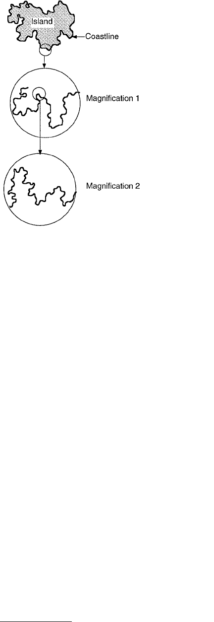
FIGURE 4.10 Repeated magniﬁcation of a coastline produces an

increased amount of wiggliness without any appearance of smoothness

at any scale. Note that the magniﬁcation is equal in all directions.

≈

−

where D is called the fractal dimension of the coastline. If D = 1, then the length is independent of ε and

it can be called a one-dimensional object. It is observed that this power law behavior remains unchanged

over several decades of length scales such that the value of D, which in some sense measures the wiggliness

of the curve, remains constant and independent of ε. Therefore, D is one parameter that can be used to

characterize a coastline. Another way of looking at this behavior is the following — although the coastline

seems a rather convoluted and complex geometric structure, the power law behavior represents a pattern

or order in this chaotic structure.

4.3.3.2 Fractal Characterization of Surface Roughness

The same concept can be used to characterize a rough surface. However, there is a difference between a

coastline and a rough surface. To show the self-similarity of a coastline, one needs to take a small part

and enlarge it equally in all directions to resemble the full coastline statistically, as qualitatively shown

in Figure 4.9. However, for a small region of a rough surface to statistically resemble* a larger region, the

enlargement should be done unequally in the vertical (z) and lateral (x and y) directions. Such objects,

which scale differently in different directions, are called self-afﬁne (Mandelbrot, 1982, 1985; Voss, 1988).

To characterize a self-afﬁne object one cannot use the length of the surface proﬁle or the area of the

surface as a measure

(Mandelbrot, 1985). There are two other ways to characterize it — the power

spectrum P(ω) and the structure function, S(τ).

4.3.3.2.1 Power Spectrum

Consider a surface proﬁle, z(x) in the x-direction. The power spectrum of the proﬁle can be found by

the relation (Blackman and Tuckey, 1958; Papoulis, 1965):

(4.3.12)

where the coordinate x ranges from 0 to L. The power spectrum can be obtained from a measured

roughness proﬁle by a simple fast Fourier transform routine

(Press et al., 1992). The square of the

amplitude of z(x) or the power at a frequency ω is equal to P(ω)dω. The rms height, the rms slope, and

the rms curvature can be obtained from the power spectrum (McCool, 1987; Majumdar and Bhushan,

1990):

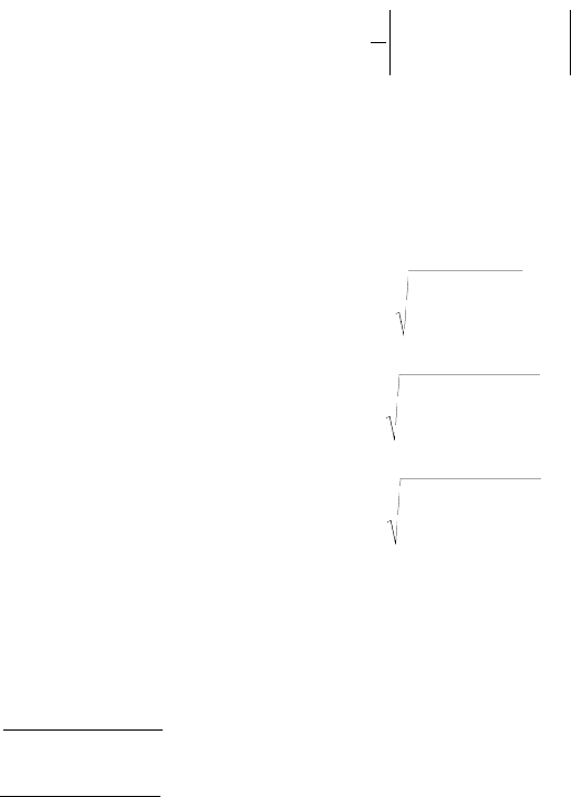
(4.3.13)

(4.3.14)

(4.3.15)

where ω

and ω

are the low-frequency and the high-frequency cutoffs, respectively. For a roughness

measurement, the low-frequency cutoff is equal to the reciprocal of the sample length, ω

= 1/L and the

high-frequency cutoff is equal to the Nyquist frequency or equal to ω

= ½τ, where τ is the distance

between two adjacent points of the data sample. It is evident that the power spectrum is a more

*Statistical resemblance is for the power spectrum or structure function of the rough surface as shown later.

zx i x dx

ωω

()

() ( )

∫

exp

σωω

()

∫

′

()

∫

σωωω

′′

()

∫

σωωω

fundamental quantity than the rms values since the rms values can be obtained from the spectrum, and

not vice versa.

For a fractal surface proﬁle, the power spectrum follows a power law of the form (Mandelbrot, 1982;

Voss, 1988; Majumdar and Tien, 1990; Majumdar and Bhushan, 1990):

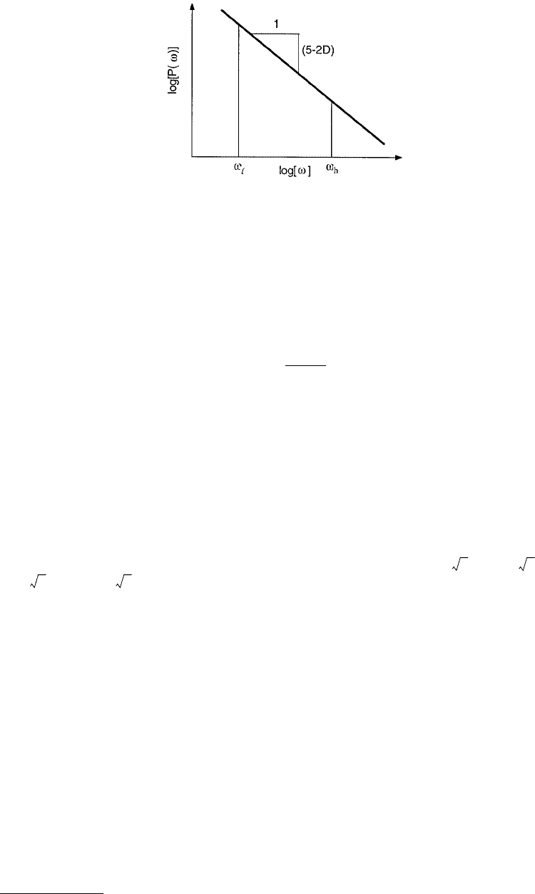
(4.3.16)

where 1 < D < 2 is the fractal dimension of the proﬁle and C is a scaling constant, which depends on

the amplitude of the rough surface. If the power spectrum of a measured surface proﬁle is found and

plotted against the frequency in a log–log plot, then the surface proﬁle can be called fractal if the spectrum

follows a straight line, as qualitatively shown in Figure 4.11. The dimension D can be obtained from the

slope and the constant C from the power. Since the proﬁle is a vertical cut through a surface, the dimension

of the surface, D

is equal D

= D + 1 only for an isotropic surface. For anisotropic surfaces one needs to

determine the fractal dimensions of surface proﬁles in different directions. For a fractal proﬁle, the

independence of D and C from the length scale ω make them unique to a surface and can therefore be

used for roughness characterization. When the rms quantities are obtained from the fractal spectrum by

using Equations 4.3.13 through 4.3.15), they exhibit the following behavior: σ = ω

–(2–D)

= L

(2–D)

;

σ′ = ω

(D–1)

; σ″ = ω

. It is evident that the rms values depend either on the low-frequency or high-

frequency cutoff and are therefore scale dependent. Figures 4.6 and 4.7 conﬁrm this experimentally and,

in fact, show the decrease in exponent by 1 as we go from the rms curvature to the rms slope and ﬁnally

to the rms height. The only difference that one ﬁnds in the rms quantities is that the rms slope and the

curvature depend on the high-frequency cutoff, whereas the rms height depends on the low-frequency

cutoff. The relation σ ≈ L

(2-D)

is exactly the same as suggested in Equation 4.3.8 with n = 2(2 – D). In

fact, the relation suggested by Sayles and Thomas (1978) in Equation 4.3.6 is a special case when D = 1.5.

The variance of the height distribution, σ

, is equal to the area under the power spectral curve as

mathematically shown in Equation 4.3.13. When the variance (or the rms height) is independent of the

sample size or any length scale, as demonstrated in Figure 4.6, the area under the power spectrum must

be constant and independent of ω

and ω

. Therefore, the fractal power law variation of the spectrum in

Equation 4.3.16 is clearly not valid for such a case since it always leads to ω

-dependence of the rms

height. One must note, then, that the fractal behavior is not followed all the time.

One of the practical difﬁculties of using the power spectrum to obtain the values of D and C is that

for a single measured roughness proﬁle, the calculated spectrum turns out to be very noisy. This is because

the roughness proﬁle is not bandwidth limited and is in fact a broad-band spectrum. However, the power

spectrum of any measured roughness will be limited to the Nyquist frequency ω

, on the high-frequency

FIGURE 4.11 Qualitative description of a fractal power spectrum plotted on a log–log plot. Note that the spectrum

is a straight line whose slope depends on the fractal dimension. A roughness measurement contains a lower, l, and

upper limit, L, of length scales which correspond to the frequency window between ω

= 1/L and ω

= 1/(2l).

()

−

()

C C

side. This gives rise to the problem of aliasing

(Press et al., 1992) which falsely translates the power of

frequencies in the range ω > ω

into the range ω < ω

. The problem comes about due to the discreteness

of the roughness measurement. To overcome this problem, we have found that the structure function

can yield more accurate estimation of D and C.

4.3.3.2.2 Structure Function

The structure function (Mandelbrot, 1982; Voss, 1988) is deﬁned as

(4.3.17)

The summation on the right-hand side can be used for calculation of a measured surface proﬁle con-

taining N points. As one can see, the structure function is easy to calculate since it does not involve any

transformation but simple height differences and averages. It is sometimes used in experimental and

theoretical analysis of velocity and scalar ﬂuctuations in turbulent ﬂuid dynamics

(Kolmogoroff, 1941).

In turbulence, the ﬂuctuating quantity varies with time and space, whereas for rough surface, the same

varies with space. The problems are quite similar since in turbulence, too, the power spectrum of the

ﬂuctuations is broadband and follows the power law behavior of Equation 4.3.16.

It is interesting to note that in some ways the structure function and the variance, σ

, of height in

Equation 4.3.4 are similar since both involve ﬁnding the average of the square of height differences.

However, the structure function uses height differences with points separated by a distance τ, whereas

for the variance, the height differences are with the mean height z

. The structure function yields much

more information than the rms height since by varying τ, one can study the roughness structure at

different length scales. This is, of course, not possible for the variance, σ

, which ﬁnds the average height

difference from the mean over the whole surface. In addition, the variance of the proﬁle slope, S′(τ), can

be found as

(4.3.18)

A surface proﬁle is said to be fractal if the structure function follows a power law behavior

as (Man-

delbrot, 1985; Voss, 1988; Majumdar et al., 1991)

(4.3.19)

This can also be derived from the power spectrum by the relation (Berry, 1978)

(4.3.20)

where D is the fractal dimension and G is a scaling constant that has units of length. When S(τ) is plotted

against τ on a log–log plot, the curve will be a straight line for a fractal proﬁle. The dimension can be

obtained from the slope and G from the intercept at a certain value of τ. The two characterization

parameters, D and G, are unique for a fractal proﬁle and are independent of any length scale τ. Thus,

they form the fundamental set of parameters for a rough surface proﬁle. By using the fractal power law

spectrum of Equation 4.3.16 in Equation 4.3.20, the structure function becomes

(Berry, 1978)

zx zx dx

zx zx

ττ

()

−

()

[]

−

()

−

()

[]

∫

∑

−

()

∆

′

()

−

()













()

∫

zx zx

ττ

()

−

()

−

()

2122

SPidτ ω ωτ ω

()

() ( )

−

[]

−∞

∞

∫

exp 1

(4.3.21)

such that the factor C of the power spectrum is related to the scaling constant G of the structure function as

(4.3.22)

Berry and Blackwell (1981) follow a slightly different deﬁnition of a fractal surface — a surface proﬁle

is said to be a self-afﬁne fractal when

(4.3.23)

where the parameter G is called “topothesy” following the term coined by Sayles and Thomas

(1978).

This deﬁnition is valid in the limit τ→0 and the fractal dimension D so obtained is called the Haus-

dorff–Besicovitch dimension

(Mandelbrot, 1982). For larger-scale roughness, Berry and Blackwell (1981)

suggest a simple model for S(τ) as

(4.3.24)

As τ→0, Equation 4.3.24 is recovered and when τ  G(2σ/G)

1/(2–D)

, S(τ) = 2σ

. In this case it is assumed

that the rms height, σ, is independent of the sample size and can be obtained from roughness data for

a sample size larger than the correlation length, τ

= G(2σ/G)

1/(2–D)

. Experimental data will show that the

behavior of Equation 4.3.24 is followed by several surfaces and can be used as a good model for surfaces.

However, if the rms height is scale dependent, as observed by Sayles and Thomas

(1978), then the model

breaks down.

In the rest of the chapter the structure function will be used to study the statistical properties of rough

surfaces. This is due to its simplicity of use and the roughness information it reveals at different length

scales.

4.3.3.3 Roughness Measurements

Typically, roughness between 1 cm to about 10 µm is measured by stylus proﬁlometers, between 500 and

1 µm by optical interferometry and between 100 µm and 1 Å by scanning tunneling or atomic force

microscopy. The overlaps in the length scales between these instruments are used to corroborate the

roughness measured by different techniques.

4.3.3.3.1 Stylus Proﬁlometry

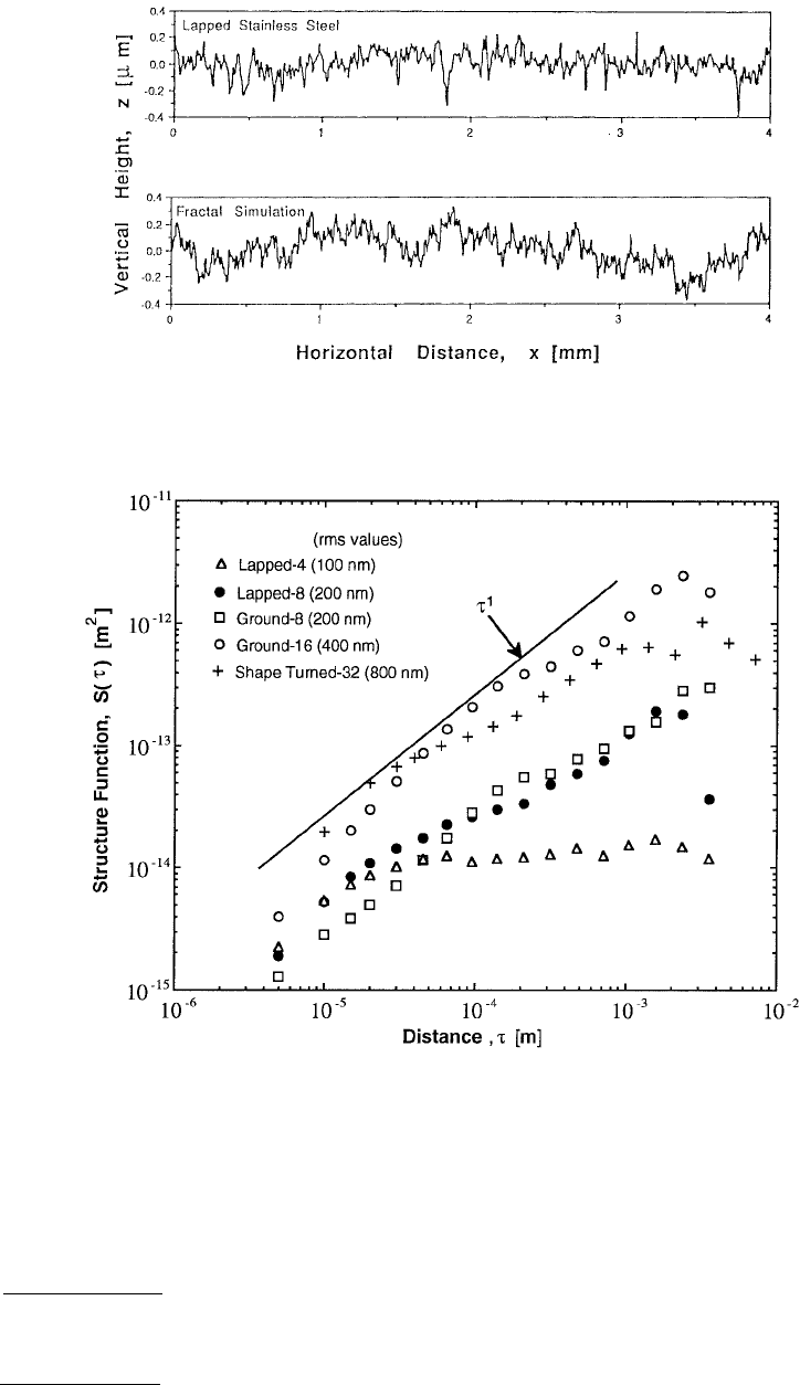
The roughness of machined (lapped, ground, and shape turned) stainless steel surfaces was measured by

a contact stylus proﬁler

(Majumdar and Tien, 1990). The instrument used a diamond stylus of radius

2.5 µm and had a vertical resolution of 0.5 nm. The scan lengths ranged from 50 to 30 mm with each

scan having 800 to 1000 evenly spaced points. Figure 4.12 shows the roughness proﬁle of a lapped stainless

steel surface.

The structure functions, S(τ), of these surface proﬁles are plotted on a log–log plot in Figure 4.13.

Also shown is the straight line, S(τ) ≈ τ

, which corresponds to a fractal dimension of D = 1.5. It is

ττ

()

−

()

π−

()













−

()

−

()

sin Γ

−

()

π−

()













−

()

−

()

sin Γ

ττ τ

()

=→

−

()

−

()

2122

0 for

τσ

()

=−−

























−

()

−

()

2122

exp

evident that the experimental structure functions do follow a power law at small length scales. In fact,

although they do not coincide, they all tend to follow the same slope, that of D = 1.5. The higher value

of S(τ) for the rougher surfaces leads to a higher value of G. The structure function for the lapped-4*

FIGURE 4.12 Proﬁle of lapped stainless steel surface measured by a stylus proﬁlometer. Fractal simulation of the

proﬁle was conducted by the Weierstrass–Mandelbrot function. (From Majumdar, A. and Tien, C. L. (1990), Wear

136; 313–327. With permission.)

FIGURE 4.13 Structure function of machined stainless steel surfaces whose roughness was measured by stylus

proﬁlometry.

*The number associated with each process is the rms roughness produced in microinches. One microinch is equal

to 25.4 nm.