Bhushan B. Handbook of Micro/Nano Tribology, Second Edition

Подождите немного. Документ загружается.

proﬁle departs from the D = 1.5 behavior at about 30 µm and those of ground-8 and lapped-8 proﬁle

depart at about 100 µm. This behavior is probably due to the following reason. For any machining process,

there exists a critical length scale below which the surface remains unaffected during machining. For

grinding, this length scale is the grain size of the abrasive material, whereas for turning it is the tool

radius. Below this scale, the surface is formed by a natural process such as fracture. This natural process

seems to lead to the same type of surface fractal behavior with D = 1.5. At length scales larger than the

critical one, the machining processes ﬂattens the surface and thus reduces the height differences between

two points on the surface. Thus, the structure function decreases at larger scales. As shown earlier, the

rms height depends on the total length, L, of the roughness sample as σ ≈ ω

D–2

= L

2–D

. Although the

structure function of the different surface proﬁles at small length scales are nearly the same, their rms

heights are quite different. This is because at larger length scales, which control the value of σ, the

structure functions are different with smoother surfaces having smaller values of S(τ).

4.3.3.3.2 Atomic Force Microscopy

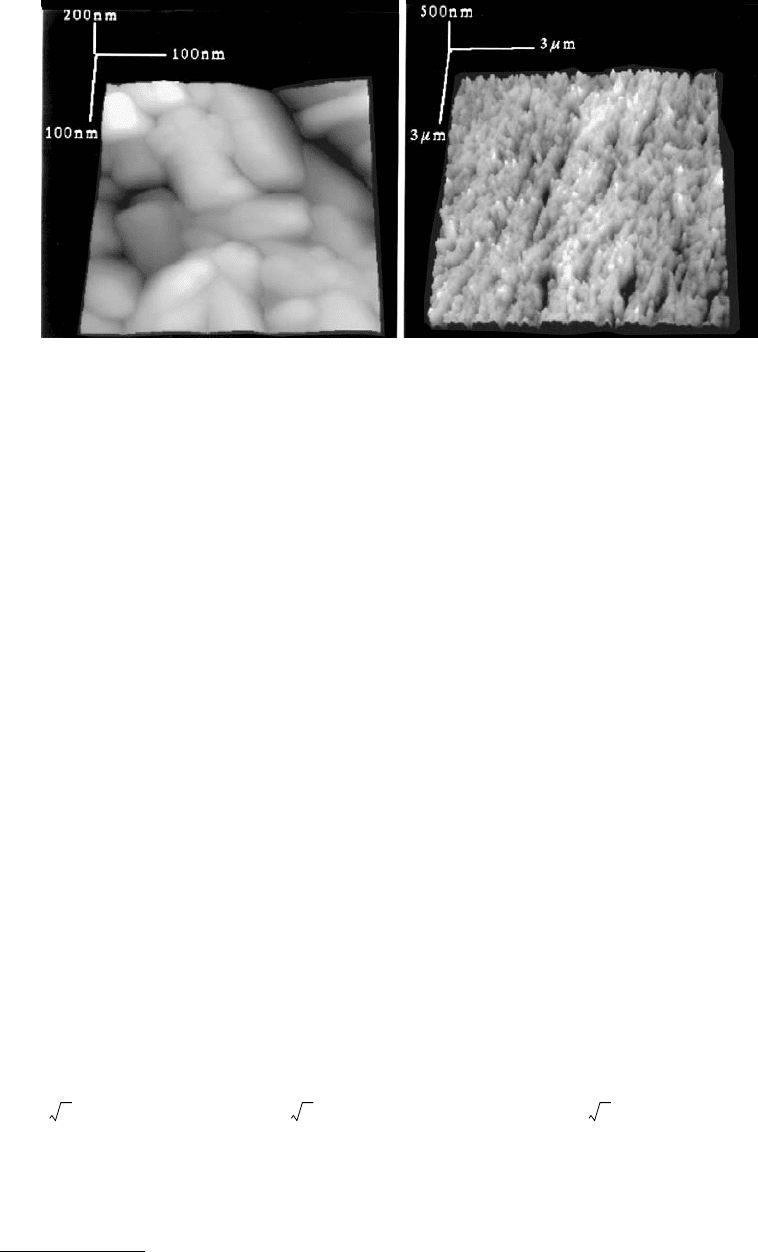
Oden et al. (1992) measured the surface roughness of magnetic tape A (Bhushan et al., 1988) at four

different resolutions by atomic force microscopy. Figure 4.14 shows the image of the tape obtained from

a 0.4 × 0.4 µm scan and 2.5 × 2.5 µm scan. The accicular magnetic particles, typically 0.1 µm in diameter

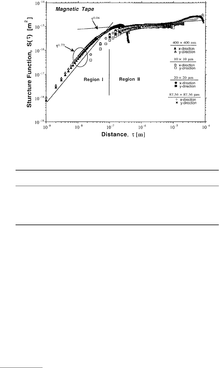
with an aspect ratio of about 10, are clearly visible. Figure 4.15 shows the structure function of all the

four scans, including the two in Figure 4.14 and for 10 × 10 µm and 40 × 40 µm scans. The overlap

between the two structure functions indicates that scan rates did not inﬂuence the roughness measure-

ment. The slight anisotropy in the x- and the y-directions correspond to the marginal bias in the

orientation of the magnetic particles along the length of the tape. It is interesting to note that the structure

function has two regions with a knee at around 0.1 µm. This suggests that the behavior S(τ) ~ τ

1.23

for

scales smaller than 0.1 µm correspond to the roughness within a single particle. The S(τ) ~ τ

behavior

for larger scales probably arise due to the fact that these particles lie adjacent to each other, much like a

single layer of pencils on a ﬂat surface. Since the diameters of the particles are nearly the same, the height

difference (z(x + τ) – z(x)) remains independent of τ for τ > 0.1 µm. The S(τ) ~ τ

behavior corresponds

to a dimension of D = 2 for surface proﬁles. This, therefore, explains the variation of rms curvature as

σ″ = ω

∝ β

, rms slope as σ′ = ω

(D–1)

∝ β

; and rms height as σ = L

(2–D)

∝ β

in Figure 4.4.

The scale independence of the rms height, and the general behavior of the structure function data of

the magnetic tape, suggests that this surface is a perfect example of the model proposed by Berry and

Blackwell

(1981), given in Equation 4.3.24 — power law behavior of D = 1.39 as τ→0 and a saturation

behavior as τ→∞.

FIGURE 4.14 Images of a magnetic tape A (Bhushan et al., 1988) surface obtained by atomic force microscopy.

Note the magnetic particles, which are oblong in shape with aspect ratio 10 and a diameter of about 100 nm.

C C C

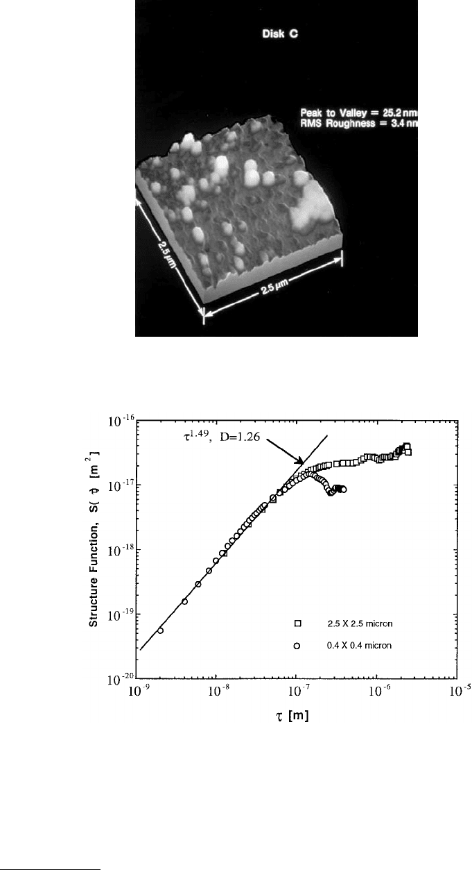
The surface topography of several magnetic thin-ﬁlm rigid disks was also studied by atomic force

microscopy

(Bhushan and Blackman, 1991). The manufacturing process for these disks are discussed by

Bhushan and Doerner (1989) and are summarized in Table 4.1. Figure 4.16 is an example of an AFM

image of magnetic disk C (Bhushan and Doerner, 1989) for which the surface is composed of columnar

grains of about 0.1 to 0.2 µm width which form during sputter-deposition. Since the substrate was

untextured, the roughness of the ﬁlms appeared quite isotropic. This is a 2.5 × 2.5 µm image which has

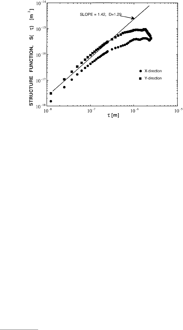
a resolution of 12.5 nm. To check whether or not surface roughness appears at even smaller scales, a

0.4 × 0.4 µm scan, having a resolution of 2 nm, was obtained for the same surface. The structure function

of the surface proﬁles for both scans revealed that roughness does appear fractal at nanometer scales as

shown in Figure 4.17. The power law behavior of S(τ) ~ τ

1.49

suggests a fractal dimension of D = 1.26

for the surface proﬁles. The structure function deviates from this power law behavior at about 0.2 µm.

It is interesting to note that this corresponds to the size of the columnar grains that are visible in the

atomic force microscopy image. Therefore, this power law behavior corresponds to intergranular surface

roughness. It is difﬁcult to obtain any meaningful information for larger length scales when τ is compa-

rable to the sample size, L. This is because the number of data points available is not good enough for

statistical averaging required to obtain the structure function.

FIGURE 4.15 Structure function of the magnetic tape A surface.

TABLE 4.1 Construction of the Magnetic Rigid Disks

Disk Designation

Substrate

(Ni–P on Al–Mg) Construction of Magnetic Layer Overcoat

A Polished γ-Fe

particles in epoxy binder Perﬂuoropolyether (PFPE)

lubricant (liquid)

B Textured Sputtered metal ﬁlm Sputtered+ PFPE

C Polished Sputtered metal ﬁlm Sputtered+ PFPE

D Textured Plated metal ﬁlm Sputtered+ PFPE

E Polished Plated metal ﬁlm Sputtered+PFPE

From Bhushan, B. and Doerner, M. F. (1989), J. Tribol. 111, 452–458. With permission.

Figure 4.18 shows the structure function for a particulate disk. Note the vertical scale is higher than

that of Figure 4.17, suggesting that the particulate magnetic disk A is much rougher than the sputter-

deposited one. In this case again, the power law behavior at smaller scales suggests a fractal behavior.

Deviations at larger length scale could be due to nonfractal characteristics or lack of statistical average.

FIGURE 4.16 Surface image of magnetic rigid disk C (Bhushan and Doerner, 1989) obtained by atomic force

microscopy (Bhushan and Blackman, 1991).

FIGURE 4.17 Structure function of the magnetic rigid disk C surface.

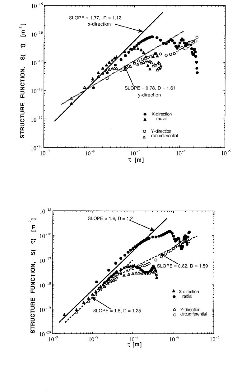
Figure 4.19 shows the structure function for magnetic rigid disk B which is textured in the circumferential

direction. The magnetic thin ﬁlms were sputter-deposited on the textured substrate. Note the differences

in the structure function in the circumferential and radial directions. The proﬁle in the radial direction

goes across all the quasi-periodic texture marks, which leads to oscillations in the structure function.

Such oscillations cannot be modeled by fractals and must be handled by a more general technique, as

discussed in Section 4.3.4. Figure 4.20 shows the structure function of the textured magnetic rigid disk

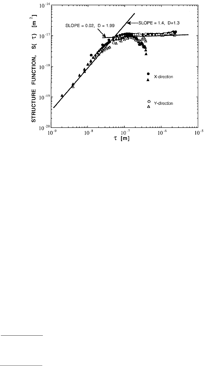
D, whereas Figure 4.21 shows that of the untextured rigid disk E. In both these cases the magnetic thin

ﬁlms were electroless plated on to the substrate. Note that the data levels off for τ > 50 nm, which is

probably a characteristic length scale for the plating process.

It is clear from the structure function data that there normally exists a transition length scale, l

which demarcates two regimes of power law behavior. At scales smaller than l

, the fractal power law

behavior is generally followed for all of the surfaces. At larger length scales, the structure function of the

polished (or untextured) disks either saturates such that the Berry–Blackwell model can be easily applied

or, in some cases, it follows a different power law behavior that can be characterized by another fractal

dimension. If the surface is textured, however, the structure function at larger length scales oscillates and

does not follow a scaling power law behavior. Such nonfractal behavior cannot be characterized by the

fractal techniques and a more general method is needed. This is discussed in detail in Section 4.3.4. The

transition length scale, l

, usually corresponds to a surface machining or growth process. For polycrys-

talline surfaces this may be the grain size, whereas for machining it is the characteristic tool size.

Recent experiments by Ganti and Bhushan (1995) showed that when a surface is imaged with atomic

force microscopy and an optical proﬁler, values of D of a wide variety of surfaces fall in a close range

but the values of G can vary a lot for the same surface. This is in contrast with the data presented above.

However, the check for reliable data is to see whether or not the structure functions of the roughness

measured at different resolutions and by different instruments overlap over common length scales.

Inspection of their data showed that although the structure functions of the atomic force microscopy

measurements of different scan sizes for the same surface seem to overlap over the common length scales,

there was large discrepancy between the structure functions obtained from atomic force microscopy and

optical proﬁler data. Therefore, it is inconclusive whether the discrepancy is due to the measurement

technique or due to the characterization method.

FIGURE 4.18 Structure function of a particulate magnetic rigid disk A (Bhushan and Doerner, 1989) whose surface

roughness was measured by atomic force microscopy.

FIGURE 4.19 Structure function of magnetic rigid disk B (Bhushan and Doerner, 1989). The magnetic thin ﬁlms

were sputter-deposited on a textured substrate. The triangles are for a 0.8 × 0.8 µm atomic force microscopy scan

containing 200 × 200 points. The circles are for a 2 × 2 µm atomic force microscopy scan containing 200 × 200 points.

FIGURE 4.20 Structure function of textured magnetic rigid disk D (Bhushan and Doerner, 1989) in which the

magnetic thin ﬁlms were electroless plated on to the substrate. The triangles are for a 0.4 × 0.4 µm atomic force

microscopy scan containing 200 × 200 points. The circles are for a 2.5 × 2.5 µm atomic force microscopy scan

containing 200 × 200 points.

It is evident that fractal characterization is valid in certain regimes of surface length scales. In these

regimes, the fractal techniques prove to be superior to conventional characterization techniques that use

rms values. It is therefore instructive to understand what the fractal parameters D and G really mean.

4.3.3.4 What Do D and G Really Mean?

Since a rough surface is self-afﬁne, thereby scaling differently in the two orthogonal directions, it needs

two parameters for characterization. These are D and G. At this point, the reader may ask what do a

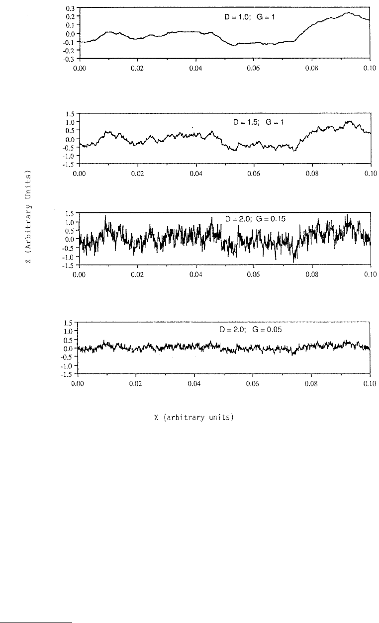
surface proﬁles look like for different values of D and G. Figure 4.22* shows that when D is close to unity,

the proﬁle is smooth having more amplitude for long wavelength undulations and low amplitude for

short wavelength undulations. As D is increased, the proﬁle gets more wiggly and jagged. When D reaches

close to 2, the proﬁle becomes nearly space ﬁlling and therefore more like a surface. Therefore, a decrease

in D effectively stretches the proﬁle along the lateral direction and therefore changes the spatial frequency.

So the value of D controls the relative amplitude of roughness at different length scales. In contrast, an

increase in G stretches the curve in the vertical direction as shown in Figure 4.22. So the value of G

controls the absolute amplitude of the roughness over all length scales.

The concept of roughness and smoothness, as discussed in Section 4.2.1, becomes quite ambiguous

under these conditions. Should a surface with a higher G, and thus more amplitude, be called rougher

or should a surface with higher D, and therefore more jagged, be called rougher? The problem is that

the concepts of rough and smooth are too crude to distinguish between amplitude variations and

frequency variation (or jaggedness) and so it is difﬁcult to say which can be called rougher or smoother.

It could be a combination of both, but at present it is unknown what this combination is.

FIGURE 4.21 Structure function of untextured magnetic rigid disk E (Bhushan and Doerner, 1989) in which the

magnetic thin ﬁlms were electroless plated on a polished substrate. The triangles are for a 0.4 × 0.4 µm atomic force

microscopy scan containing 200 × 200 points. The circles are for a 2.5 × 2.5 µm atomic force microscopy scan

containing 200 × 200 points.

*These are fractal simulations of rough surfaces obtained by using the Weierstrass–Mandelbrot function. Details

of the simulation procedure is discussed in detail elsewhere

(Voss, 1988; Majumdar and Bhushan, 1990; Majumdar

and Tien, 1990).

4.3.3.5 rms Values and D and G

The rms parameters, σ, σ′, and σ″ have been used extensively in the tribology literature and therefore

researchers are more familiar with them. Although they show scale-dependent characteristics, it is instruc-

tive to know how they relate to fractal characterization parameters D and G. The rms parameters are

related to the power spectrum as shown in Equations 4.3.13 through 4.3.15.

Consider the rms height, σ, ﬁrst. If σ is scale independent, then the model of Berry and Blackwell

(1981) for the structure function as given in Equation 4.3.24 is valid. In this case, G and D correspond

to the limit of τ→0, whereas σ corresponds to the scales much larger than the correlation length τ

. In

other words, the rms height is unrelated to the fractal parameters G and D since the structure function

does not follow the same behavior in the two limits.

FIGURE 4.22 Effect of varying D and G on the proﬁles of rough surfaces. These are simulations (Majumdar and

Tien, 1990) of rough surfaces obtained from the Weierstrass–Mandelbrot function. The effect of increasing D is to

make the proﬁle more jagged, or in other words, a lateral compression. An increase in G increases the amplitude of

roughness over all length scales.

The scale dependence of the rms height, σ, comes from the fractal power law variation of the power

spectrum as given in Equation 4.3.16. The variance, σ

, can be found as

(4.3.25)

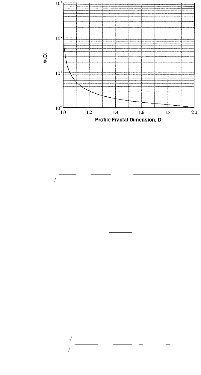
The variation of the factor

with the fractal dimension D is shown in Figure 4.23. As D→1, ψ tends to ∞, whereas when D = 2, the

ψ is equal to unity. It is clear that σ, G, and D are related in a complicated manner. But what is important

is that σ does not depend on the instrument resolution but on the sample length, L. If σ is obtained for

a wide range of varying sample length, L, then the fractal dimension D can be found from the slope of

the log–log plot of σ vs. L. Once the D is found, the factor ψ can be found from Figure 4.23. With D

and ψ known, the scaling constant G can be obtained from the relation in Equation 4.3.25. If the structure

function or the power spectrum follows different power laws in different length scales, Equation 4.3.25

must be modiﬁed. This is discussed in Appendix 4.1.

The relation between rms slope, σ′, and the fractal parameters G and D can also be obtained from

the power spectrum as follows:

(4.3.26)

FIGURE 4.23 Variation of the factor ψ(D) with the proﬁle fractal dimension D.

2122

−

()

π−

()













−

()

−

()

∞

−

()

−

()

−

()

∫

sin Γ

ΨΓD

()

π−

()













−

()

sin

′

−

()

−

()













−

























∫

−

()

−

()

21 21

52 2 1

11C

where l is the smallest length scale that is measured by the instrument. For D > 1 and L  l,

Equation 4.3.26 can be simpliﬁed to

(4.3.27)

It is clear that the rms slope does not depend on the sample length, L, but on the instrument resolution,

l as σ′ ≈ l

–(D–1)

. For the limiting case, D → 1, we ﬁnd that ψ(D) → 1/2(D – 1) such that the denominator

in Equation 4.3.27 is equal to unity. For a surface with multifractal regimes, see Appendix 4.1 for the rms

slope.

The rms curvature, σ″, can be found similarly as

(4.3.28)

where it is assumed that L  l. It is evident that σ″ ≈ l

–D

such that it depends only on the instrument

resolution and not on the sample length, L.

The autocorrelation function is also often used to characterize rough surface proﬁles. The relation

between the autocorrelation function and the fractal parameters D and G are given in Appendix 4.2.

4.3.3.6 Asperity Geometry from Fractal Characteristics

One of the advantages of using the fractal roughness characterization and, in particular, the structure

function technique is that the geometric shape of asperities can be described at all length scales in the

fractal regime. Thus, for an asperity that has a base diameter of l, the height of the asperity, δ, follows

from the structure function as

(4.3.29)

Here the diameter l is used as a characteristic length scale such that the area, a, of the asperity base can

be written as, a = l

. The geometry is schematically shown in Figure 4.24 for different length scales l. If

the shape is assumed spherical, the radius of curvature, R, for the asperities can be found to follow the

relation

(4.3.30)

Thus the surface can be imagined to be a collection of asperities where small asperities are mounted on

larger asperities that are in turn mounted on larger asperities in a hierarchical manner. Once the geometric

structure is determined, the mechanics of contact and the surface force interactions can be modeled.

FIGURE 4.24 Geometry of an asperity from a fractal surface of

proﬁle dimension D. The asperities are modeled as hemispheres

with radius R and base diameter, l, such that the base area is equal

to a = l

′

−

()

−

()()













−

()

′′













−

























≈

−

()













−

()

∫

DDG

DD D

δ= =

−

()

−

()

−

()

−

()

GGa

DDDD12 12 2

−

()

−

()

4.3.4 Generalized Technique for Fractal and Nonfractal Surfaces

The fractal characterization techniques, discussed in detail in Section 4.3.3, overcome some of the short-

comings of conventional methods that use σ, σ′, and σ″. One of the requirements of the fractal technique

is that the structure function or the power spectrum must follow power law scaling behavior, that is,

S(τ) ≈ τ

2(2–D)

or P(ω) ≈ ω

–(5–2D)

. If this is satisﬁed, then the asperity height, δ, and the base size, l, follow

the scaling relation δ ≈ l

(2–D)

. This is particularly useful in tribology since only two parameters, G and

D, need to be known to study tribological phenomena at all length scales in the fractal regime. However,

the experimental data in Figures 4.13 and 4.15 through 4.21 show that although the scaling behavior is

followed in some cases, it is not universal. In addition, the power law can change at a transition length

scale and is not universal over all length scales. Yet, the rms slope and curvature cannot be used to

characterize them since the surface can have multiple scales, which, although they do not follow the

scaling behavior δ ≈ l

(2–D)

, can lead to scale-dependent rms values. A technique must therefore be

developed that will work for both fractal and nonfractal surfaces and yet be scale independent. This

section introduces a new method with these issues in mind.

It is necessary to identify ﬁrst how the surface characteristics will be used. As discussed in Section 4.2,

knowledge of the surface structure is important for predicting the size and spatial distributions of contact

spots as well as for the mechanics of asperity sliding. Since these spots are formed by asperities, what is

important is the asperity geometry at relevant length scales and its size and spatial distributions on the

surface. The conventional techniques, which use rms height, slope and curvature, ﬁnd an average asperity

shape, whereas the fractal techniques determine the shape at all length scales by the scaling law. Both

techniques can be combined to form a general method for roughness characterization as follows.

The roughness is characterized by two parameters — V(l) and K(l) — which are found in the x- and

y-directions* by the following relations.

(4.3.31)

(4.3.32)

Here the 〈〉 symbol implies averaging over the measured data points. It is evident that the function

V(l) is the square root of the structure function S(l). For a fractal surface V(l) = G

(D–1)

(2–D)

. The function

K(l) is the rms curvature of asperities of lateral scale l which in the fractal model is assumed to vary as

K(l) = G

(D–1)

. In the generalized model, such power laws will not be assumed and instead the raw data

*The x- and y-directions are chosen to be the principal directions of an anisotropic surface. The principal directions

can be found by ﬁrst obtaining V in all directions to get a V vs. l surface. If one takes a horizontal cut of the surface

for V = constant, then one can connect the loci of the intersecting l values into a curve which in general can be

approximated by an ellipse. Then the x- and the y-directions correspond to the major and the minor axes of the

ellipse. The assumption made in this model is that the major and minor axes remain the same at all length scales.

Vzxyzxy

()

−

()

[]

()

−

()

[]

zx y zx y

zx y zx y zx y

()

+−

()

[]

()

+−

()

−

()

[]

,, ,