Bielajew A.F. Fundamentals of the Monte Carlo method for neutral and charged particle transport
Подождите немного. Документ загружается.

17.1. ELECTRON-SPECIFIC METHODS 281
17.1.3 PRESTA!
In the previous Chapter 14, Electron step-size dependencies and PRESTA, we discussed an
alternative electron transport algorithm, PRESTA. This algorithm, by making improvements
to the physical modeling of electron transport, allows the use of large electron steps when one
is far away from boundaries. This algorithm may, therefore, be considered to be a variance
reduction technique, since it saves computing time by employing small steps only where
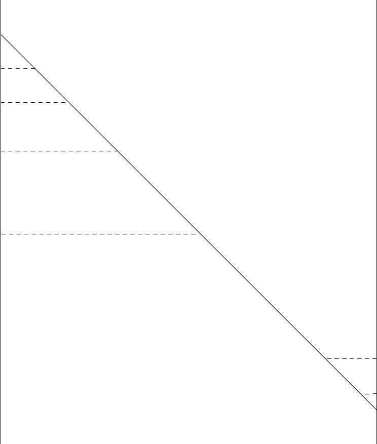
needed—in the vicinity of boundaries and interfaces, as depicted in figure 17.3. Continuing
with the present example, we calculate the gain in efficiency ratio, (PRESTA)/(base), to
be 6.1. RIG is always switched on with PRESTA, so it is actually fairer to calculate the
efficiency ratio, (PRESTA)/(RIG), which was found to be 4.6. If we allow zonal discard as
well, we calculate the efficiency ratio, (zonal discard + PRESTA)/(zonal discard + RIG),
to be 3.1. There is a brief discussion in the previous chapter on when PRESTA is expected
to run quickly. Basically, the fewer the boundaries and the higher the transport cutoffs, the
faster PRESTA runs. A detailed discussion is given in the PRESTA documentation [BR87].
17.1.4 Range rejection
As a final example of electron variance reduction, we consider the technique called “range
rejection”. This is similar to the “discard within a zone” except for a few differences. Instead
of discarding (i.e. stopping the transport and depositing the energy “on the spot”) the
electron because it can not reach the boundaries of the geometrical element it is in, the
electron is discarded because it can not reach some region of interest. This is depicted
in figure 17.4. For example, a particle detector may contain a sensitive volume where one
wishes to calculate energy deposit, or some other quantity. Surrounding this sensitive volume
may be shields, converters, walls etc. where one wishes accurate particle transport to be
accomplished but where one does not wish to score quantities directly. Electrons that can
not reach the sensitive volume may be discarded “on the spot”, providing that the neglect
of the bremsstrahlung γ’s causes no great inaccuracy.
As an example of range rejection, we consider the case of an ion chamber [BRN85]. In
this case, a cylindrical air cavity, 2 mm in depth and 1.0 cm in radius is surrounded by 0.5
g/cm
2
carbon walls. A flat circular end is irradiated by 1.25 MeV γ-rays incident normally.
This approximates the irradiation from a distant source of
60
Co. This is a “thick-walled”
ion chamber, so-called because it’s thickness exceeds the range of the maximum energy
electron that can be set in motion by the incident photons. This sets up a condition of
“near charged particle equilibrium” in the vicinity of the cavity. The potential for significant
saving in computer time is evident, for many electrons could never reach the cavity. We
are interested in calculating the energy deposited to the air in the cavity and we are not
concerned with scoring any quantities in the walls. The range rejection technique involved
calculating the closest distance to the surface of the cavity on every transport step. If this
distance exceeded the CSDA range of the electron, it was discarded. The omission of residual
282 CHAPTER 17. VARIANCE REDUCTION TECHNIQUES
x
x
x
start
Boundary
Boundary
x
x
x
x
end
Figure 17.3: A depiction of PRESTA-like transport for the diagonal trajectory discussed
previously.
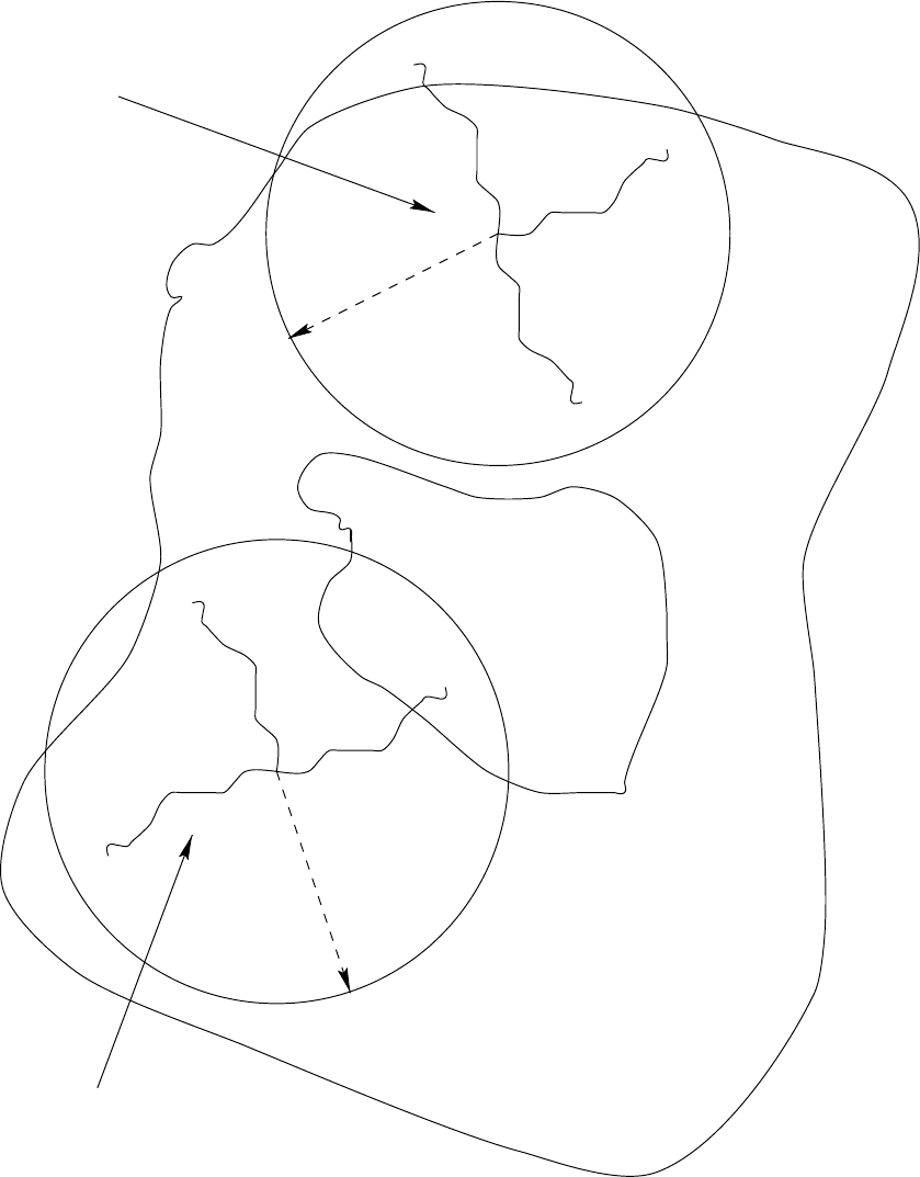
17.1. ELECTRON-SPECIFIC METHODS 283
no scoring in
this region
region of
interest
score
here
range discard
these electrons
fully transport
these electrons
R(E)
R(E)
Figure 17.4: A depiction of range rejection.

284 CHAPTER 17. VARIANCE REDUCTION TECHNIQUES
bremsstrahlung photon creation and transport was negligible in this problem. The secondary
particle creation thresholds were set at 10 keV kinetic energy as well as the transport cut-off
energies. (ECUT=AE=0.521 MeV, PCUT=AP=0.01 MeV, and ESTEPE=0.01 for accurate
low energy simulation.) A factor of 4 increase in efficiency was realised in this case.
Range rejection is a relatively crude but effective method. The version described above
neglects residual bremsstrahlung and is applicable when the discard occurs in one medium.
The bremsstrahlung problem could be solved by forcing at least some of the electrons to pro-
duce bremsstrahlung. The amount of energy eventually deposited from these photons would
have to be weighted accordingly to keep the sampling game “fair”. Alternatively, one could
transport fully a fraction, say f, of the electrons and weight any resultant bremsstrahlung
photons by 1/f. The other problem, the one of multi-media discard, is difficult to treat in
complete generality. The difficulty is primarily a geometrical one. The shortest distance to
the scoring region is the shortest geometrical path only when the transport can occur in one
medium. The shortest distance we need to calculate for range rejection is the path along
which the energy loss is a minimum. It is not difficult to imagine that finding the “shortest”
path for transport in more than one medium may be very difficult. For special cases this
may be done or approximations may be made. The “payoff” is worth it as large gains in
efficiency may be realised, as seen in the above example.
17.2 Photon-specific methods
17.2.1 Interaction forcing
In problems where the interaction of photons is of interest, efficiency may be lost because
photons leave the geometry of the simulation without interacting. This is depicted in fig-
ure 17.5 where an optically thin region (one for which µt is small, where t is the thickness of
the slab and µ is the interaction coefficient) allows many photons to penetrate and escape
the region. Efficiency is lost because time is spent tracking photons through a geometry and
they do not contribute to the score. This problem has a simple and elegant solution.
The probability distribution for a photon interaction is:
p(λ)dλ = e
−λ
dλ, (17.3)
where 0 ≤ λ<∞ and λ is the distance measured in mean free paths. It can easily be shown
that sampling λ from this distribution can be accomplished by the following formula
2
:
λ = −ln(1 − ξ), (17.4)
2
It is conventional to use the expression, λ = −ln(ξ), since both 1 −ξ and ξ are distributed uniformly on
(0,1) but the former expression executes more slowly. However, it has a closer connection to the following
mathematical development.
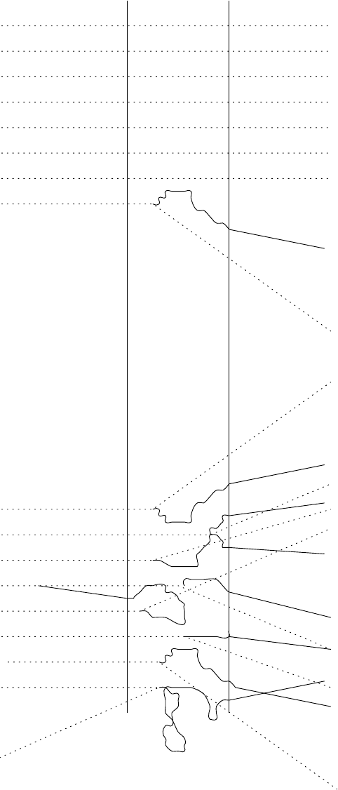
17.2. PHOTON-SPECIFIC METHODS 285
Interaction forcing
unforced
"wasted"
photons
forced
thin
region
every
photon
contributes
vacuum vacuum
optically
Figure 17.5: A depiction of photon interaction forcing.

286 CHAPTER 17. VARIANCE REDUCTION TECHNIQUES
where ξ is a random number uniform on the range, 0 ≤ ξ<1. Since λ extends to infinity
and the number of photon mean free paths across the geometry in any practical problem
is finite, there is a non-zero and often large probability that photons leave the geometry of
interest without interacting. If they don’t interact, we waste computing time tracking these
photons through the geometry.
Fortunately, this waste may be prevented. We can force these photons to interact. The
method by which this can be achieved is remarkably simple. We construct the probability
distribution,
p(λ)dλ =
e
−λ
dλ
R
Λ
0
e
−λ
0
dλ
0
, (17.5)
where Λ is the total number of mean free paths along the direction of motion of the photon
to the end of the geometry. (The geometry may be arbitrary.) This λ is restricted to the
range, 0 ≤ λ<Λ, and λ is selected from the equation,
λ = −ln(1 − ξ(1 − e
−Λ
)). (17.6)
We see from eq. 17.6 that we recover eq. 17.4 in the limit Λ −→ ∞. Since we have forced
the photon to interact within the geometry of the simulation we must weight the quantities
scored resulting from this interaction. This weighting takes the form,
ω
0
= ω(1 − e
−Λ
), (17.7)
where ω
0
is the new “weighting” factor and ω is the old weighting factor. When interaction
forcing is used, the weighting factor, 1 − e
−Λ
, simply multiplies the old one. This factor is
the probability that the photon would have interacted before leaving the geometry of the
simulation. This variance reduction technique may be used repeatedly to force the interaction
of succeeding generations of scattered photons. It may also be used in conjunction with other
variance reduction techniques. Interaction forcing may also be used in electron problems to
force the interaction of bremsstrahlung photons.
On first inspection, one might be tempted to think that the calculation of Λ may be difficult
in general. Indeed, this calculation is quite difficult and involves summing the contributions
to Λ along the photon’s direction through all the geometrical elements and materials along
the way. Fortunately, most of this calculation is present in any Monte Carlo code because
it must possess the capability of transporting the photons through this geometry! This
interaction forcing capability can be included in the EGS code in a completely general,
geometry independent fashion with only about 30 lines of code [RB84]!
The increase in efficiency can be dramatic if one forces the photons to interact. For example,
for ion chamber calculations similar to those described in sec. 17.1.4 and discussed in detail
elsewhere [BRN85], the efficiency improved by the factor 2.3. In this calculation, only about
6% of the photons would have interacted in the chamber. In calculating the dose to skin
from contaminant electrons arising from the interaction of
60
Co (i.e. 1.25 MeV γ’s) in 100
cm of air [RB84], the calculation executed 7 times more efficiently after forcing the photons

17.2. PHOTON-SPECIFIC METHODS 287
to interact. In calculating the dose from
60
Co directly in the skin (a 0.001 cm slice of tissue)
where normally only 6 ×10
−5
of the photons interact, the efficiency improved by a factor of
2600 [RB84, RB85]!
17.2.2 Exponential transform, russian roulette, and particle split-
ting
The exponential transform is a variance reduction technique designed to enhance efficiency
for either deep penetration problems (e.g. shielding calculations) or surface problems (e.g.
build-up in photon beams). It is often used in neutron Monte Carlo work and is directly
applicable to photons as well.
Consider the simple problem where we are interested in the surface or deep penetration in
a simple slab geometry with the planes of the geometry normal to the z-axis. We then scale
the interaction probability making use of the following formula:
˜
λ = λ(1 − Cµ), (17.8)
where λ is the distance measured in the number of mean free path’s,
˜
λ is the scaled distance,
µ is the cosine of the angle the photon makes with the z-axis, and C is a parameter that
adjusts the magnitude of the scaling. The interaction probability distribution is:
˜p(λ)dλ =(1− Cµ)e
−λ(1−Cµ)
dλ, (17.9)
where the overall multiplier 1 − Cµ is introduced to ensure that the probability is correctly
normalised, i.e.
R
∞
0
˜p(λ)dλ =1. ForC = 0, we have the unbiased probability distribution
e
−λ
dλ. One sees that for 0 <C<1, the average distance to an interaction is stretched
3
.For
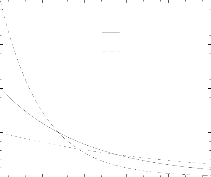
C<0, the average distance to the next interaction is shortened. Examples of a stretched
and shortened distribution are given in fig. 17.6. In order to play the game fairly, we must
obtain the appropriate weighting function to apply to all subsequent scoring functions. This
is obtained by requiring that the overall probability be unchanged. That is, we require:
ω
0
˜p(λ)dλ = ωp(λ)dλ, (17.10)
where ω
0
is the new weighting factor and ω is the old weighting factor. Solving eq. 17.10 for
ω
0
yields,
ω
0
= ωe
−λCµ
/(1 − Cµ). (17.11)
Finally, we require a technique to sample the stretched or shortened number of mean free
paths to the next interaction point from a random number. It is easily shown that λ is
selected using the formula:
λ = −ln(ξ)/(1 − Cµ), (17.12)
3
Note that the average number of mean free paths to an interaction, hλi,isgivenbyhλi =
R
∞
0
λ˜p(λ)dλ =
1
1−Cµ
.
288 CHAPTER 17. VARIANCE REDUCTION TECHNIQUES
0.0 0.5 1.0 1.5 2.0 2.5
depth/mean−free−path
0.0
0.5
1.0
1.5
2.0
Interaction probability
unbiased: C = 0
stretched: C = 1/2
shortened: C = −1
Figure 17.6: Examples of a stretched (C =1/2) and shortened (C = −1) distribution
compared to an unbiased one (C = 0). In all three cases, µ = 1. For all three curves
R
∞
0
˜p(λ)dλ is unity. The horizontal axis is in units of the number of mean free path’s (mfp’s).

17.2. PHOTON-SPECIFIC METHODS 289
where ξ is a random number chosen uniformly over the range, 0 <ξ≤ 1.
For complete generality, one must obey the restriction, |C| < 1 since the photon’s direction
is arbitrary (−1 ≤ µ ≤ 1). “Path-length stretching” means that 0 <C<1, i.e. photons are
made to penetrate deeper. “Path-length shortening” means that −1 <C<0, i.e. photons
are made to interact closer to the surface. For studies of surface regions, one may use a
stronger biasing, i.e. C ≤−1. If one used C ≤−1 indiscriminately, then nonsense would
result for particles going in the backward direction, i.e. µ<0. Sampled distances and
weighting factors become negative. It is possible to use C ≤−1 for special, but important
cases. (As we shall see in the next section, it is possible to remove all restrictions on C
in finite geometries by combining exponential transforms and interaction forcing.) If one
restricts the biasing to the incident photons which are directed along the axis of interest
(i.e. µ>0) then C ≤−1 may be used. If one uses this severe biasing, then as seen
in eq. 17.11, weighting factors for the occasional photon that penetrates very deeply can
get very large. If this photon backscatters and interacts in the surface region where one
is interested in gaining efficiency, the calculated variance can be undesirably increased. It
is advisable to use a “splitting” technique [Kah56], dividing these large weight particles
into a N smaller ones each with a new weight, ω
0
= ω/N if they threaten to enter the
region of interest. Thresholds for activating this splitting technique and splitting fractions
are difficult to specify and choosing them is largely a matter of experience with a given type
of application. The same comment applies when particle weights become vary small. If this
happens and the photon is headed away from the region of interest it is advisable to play
“russian roulette” [Kah56]. This technique works as follows: Select a random number. If
this random number lies above a threshold, say α, the photon is discarded without scoring
any quantity of interest. If the random number turns out to be below α the photon is
allowed to “survive” but with a new weight, ω
0
= ω/α, insuring the fairness of the Monte
Carlo “game”. This technique of “weight windowing” is recommended for use with the
exponential transform [HB85] to save computing time and to avoid the unwanted increase
in variance associated with large weight particles.
Russian roulette and splitting
4
can be used in conjunction with exponential transform, but
they enjoy much use by themselves in applications where the region of interest of a given
application comprises only a fraction of the geometry of the simulation. Photons are “split”
as they approach a region of interest and made to play “russian roulette” as they recede. The
three techniques, exponential transform, russian roulette and particle splitting are part of the
“black art” of Monte Carlo. It is difficult to specify more than the most general guidelines
on when they would be expected to work well. One should test them before employing them
in large scale production runs.
Finally, we conclude this section with an example of severe exponential transform biasing
with the aim to improve surface dose in the calculation of a photon depth dose curve [RB84].
4
According to Kahn [Kah56], both the ideas and terminology for russian roulette and splitting are
attributable to J. von Neumann and S. Ulam.

290 CHAPTER 17. VARIANCE REDUCTION TECHNIQUES
In this case, 7 MeV γ’s were incident normally on a 30 cm slab of water. The results are
summarised in Table 17.1. In each case the computing time was the same. Therefore,
Table 17.1: This series of calculations examines a case where a gain in the computational
efficiency at the surface is desired. Each calculation took the same amount of computing
time. In general, efficiency at the surface increases with decreased C while efficiency worsens
at depth.
C Histories Relative efficiency on calculated dose
10
3
0–0.25 cm 6.0–7.0 cm 10–30 cm
0 100 ≡1 ≡1 ≡1
-1 70 1 1.0 3.5
-3 55 1.5 1.2 0.6
-6 50 3.5 2.8 0.1
the relative efficiency reflects the relative values of 1/s
2
.AsC decreases, the calculational
efficiency for scoring dose at the surface increases while, in general, it decreases for the largest
depth bin. The efficiency was defined to be unity for C = 0 at the for each bin. For the
deepest bin there is an increase initially because the mean free path is 39 cm. At first the
number of interactions in the 10 cm–30 cm bin increases! Note that as C is deceased the
number of histories per given amount of computing time decreases. This is because more
electrons are being set it motion, primarily at the surface. These electrons have smaller
weights, however, to make the “game” fair.
17.2.3 Exponential transform with interaction forcing
If the geometry in which the transport takes place is finite in extent, one may eliminate re-
strictions on the biasing parameter, C, by combining exponential transform with interaction
forcing. By using the results of the previous two sections we find the interaction probability
distribution to be:
p(λ)dλ =
(1 − Cµ)e
−λ(1−Cµ)
1 − e
−Λ(1−Cµ)
dλ. (17.13)
The new weighting factor is:
ω
0
= ω
(1 − e
−Λ(1−Cµ)
)e
−λCµ
1 − Cµ
, (17.14)
and the number of mean free paths is selected according to:
λ = −
ln(1 − ξ(1 − e
−Λ(1−Cµ)
))
1 − Cµ
, (17.15)