Bielajew A.F. Fundamentals of the Monte Carlo method for neutral and charged particle transport

Подождите немного. Документ загружается.

4.2. REJECTION METHOD 41

−1.2

0.0

p(x

max

)

p(x)

max

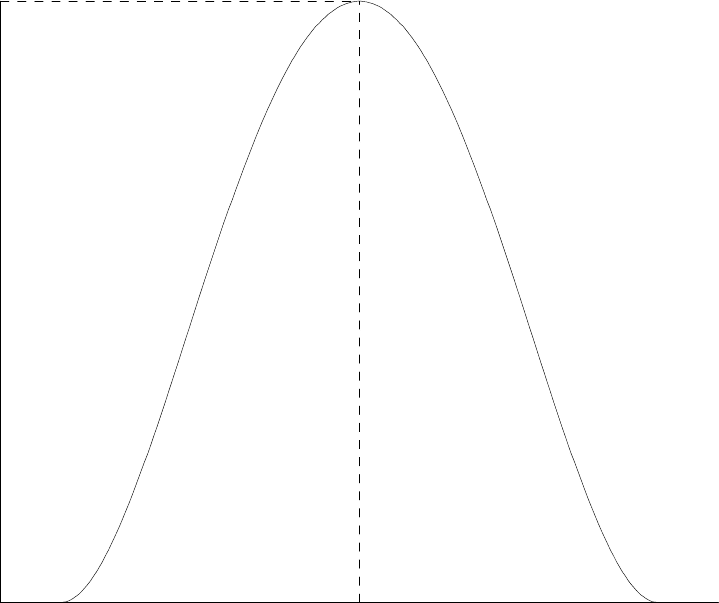
Figure 4.4: A typical probability distribution.

42 CHAPTER 4. SAMPLING THEORY

−1.2

0.0

f(x) = p(x)/p(x

max

)

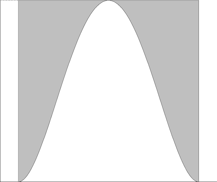
Figure 4.5: The probability distribution of Figure 4.4 scaled for the rejection technique.

4.3. MIXED METHODS 43

This method will result in x being selected according to the probability distribution func-

tion. Some consider this method “crude” because random numbers are “wasted” unlike the

invertible cumulative probability distribution function method. It is particularly wasteful for

“spiky” probability distribution functions. However, it can save computing time if the c()

−1

is very complicated. One has to “waste” many random numbers to use as much computing

time as in the evaluation of a transcendental function!

4.3 Mixed methods

As a ﬁnal topic in elementary sampling theory we consider the “mixed method”, a combi-

nation of the previous two methods.

Imagine that the probability distribution function is too diﬃcult to integrate and invert,

ruling out the direct approach without a great deal of numerical analysis, and that it is

“spiky”, rendering the rejection method ineﬃcient. (Many probability distributions have

this objectionable character.) However, imagine that the probability distribution function

can be factored as follows:

p(x)=f(x)g(x) (4.9)

where f(x) is an invertible function that contains most of the “spikiness”, and g(x)isrela-

tively ﬂat but contains most of the mathematical complexity. The recipe is as follows:

1. Normalise f(x) producing

f(x) such that

f(x)=1.

2. Normalise g(x) producing ˜g(x) such that ˜g(x) ≤ 1 ∀ x ∈ [a, b].

3. Using the direct method described previously, choose an x using

f(x) as the probability

distribution function.

4. Using this x, apply the rejection technique using ˜g(x). That is, choose a random

number, r, uniformly in the range [0, 1]. If ˜g(x) ≤ r, accept x, otherwise go back to

step 3.

Remarks:

With some eﬀort, any mathematically complex, spiky function can be factored in this man-

ner. The art boils down to the appropriate choice of

f(x)thatleavesa˜g(x)thatisnearly

ﬂat. For two recent examples of this method as applied to a production-level code, see

References [BR86] and [BMC89].

The mixed method is also tantamount to a change in variables. Let

p(x)dx = f(x)g(x)dx =(

f(x)dx)

dxf(x)

g(x) , (4.10)

44 CHAPTER 4. SAMPLING THEORY

where

f(x) is now a properly normalized probability distribution function. Employing

f(x)

as the function for the direct part, we let

u = c(x)=

f(x

)dx

, (4.11)

be a transformation between x and u. Note the limits of u,0≤ u ≤

f(x

)dx

=1. By

deﬁnition, the inverse exists so that x = c

−1

(u). As well du = f(x)dx. Thus, we can rewrite

Equation 4.10 as:

p(x)dx =

dxf(x)

g(u)du, (4.12)

which eliminates f(x) through a change in variables. Thus, one can sample g(u)using

rejection (or some other technique) and relate the selected u to x through the inverse relation

x = c

−1

(u).

If the rejection technique is employed for g(x), then the eﬃciency of is calculated in the same

way as in Equation 4.8.

4.4 Examples of sampling techniques

4.4.1 Circularly collimated parallel beam

The normalised probability distribution in this case is:

p(ρ, φ)dρ dφ =

πρ

ρ dρ dφ 0 ≤ ρ ≤ ρ

0 ≤ φ ≤ 2π (4.13)

where ρ is the cylindrical radius, ρ

is the collimation radius and φ is the azimuthal an-

gle. ρdρdφ is a diﬀerential surface element in cylindrical coordinates. This is a separable

probability distribution of the form:

p(ρ, φ)dρ dφ =dp

(ρ)dp

(φ) (4.14)

where:

(ρ)dρ =

ρ dρ 0 ≤ ρ ≤ ρ

(4.15)

and

(φ)dφ =

2π

dφ 0 ≤ φ ≤ 2π (4.16)

4.4. EXAMPLES OF SAMPLING TECHNIQUES 45

Direct method

The cumulative probability distribution functions in this case are:

(ρ)=

dρ

(4.17)

(φ)=c

(φ)=

2π

dφ

2π

(4.18)

Inverting gives:

ρ = ρ

√

(4.19)

φ =2πr

(4.20)

where the r

are random numbers on the range [0, 1].

The code segment that would produce accomplish this looks like:

rho = rho_0 * sqrt(rng())

phi = 2e0 * pi * rng()

x = rho * cos(phi)

y = rho * sin(phi)

where rng() is a function that return a random number uniformly on the range [0, 1] [or

(0, 1] or [0, 1) or (0, 1)].

Rejection method

In this technique, a point is chosen randomly within the square −1 ≤ x ≤ 1; −1 ≤ y ≤ 1. If

this point lies within a circle with unit radius the point is accepted and the x and y values

scaled by the collimation radius, ρ

. The code segment that would accomplish this looks

like:

1 x = 2e0 * rng() - 1e0

y = 2e0 * rng() - 1e0

IF (x**2 + y**2 .gt. 1e0) goto 1

x = rho_0 * x

y = rho_0 * y

46 CHAPTER 4. SAMPLING THEORY

Which is better?

Actually, both methods are equivalent mathematically. However, one or the other may have

advantages in execution speed depending on other factors in the application. If the geometry

is not cylindrically symmetric or all the scoring that is done does not make use of the inherent

cylindrical symmetry, then the rejection method is about twice as fast as the direct method

because the trigonometric functions are not employed in the rejection method.

If the geometry is cylindrically symmetric and the scoring takes advantage of this symmetry,

then the direct method is about 2–3 times faster because symmetry reduces the calculation

to:

x = rho_0 * sqrt(rng())

y=0

Many computers now have hardware square root capabilities. With this capability the direct

method may be advantageous, whether or not one makes use of the cylindrical symmetry.

4.4.2 Point source collimated to a planar circle

The normalised probability distribution in this case is:

p(θ, φ)dθdφ =

dφ

2π

sin θ dθ

1 − cos θ

0 ≤ θ ≤ θ

0 ≤ φ ≤ 2π (4.21)

where θ is the polar angle and φ is the azimuthal angle. sin θ dθ dφ is a diﬀerential solid

angle element in spherical coordinates. θ

is the collimation angle. In terms of the distance

to the collimation plane z

and the diameter of the collimation circle on this plane ρ

cos θ

= z

+ ρ

This is a separable probability distribution of the form:

p(θ, φ)dθdφ = p

(θ)dθp

(φ)dφ (4.22)

where:

(θ)dθ =

sin θdθ

1 − cos θ

0 ≤ θ ≤ θ

(4.23)

and

(φ)dφ =

2π

dφ 0 ≤ φ ≤ 2π (4.24)

The cumulative probability distribution functions in this case are:

(θ)=

1 − cos θ

sin θ

dθ

1 − cos θ

(4.25)

4.4. EXAMPLES OF SAMPLING TECHNIQUES 47

(φ)=c

(φ)=

2π

dφ

2π

(4.26)

Inverting gives:

cos θ =1−r

[1 − cos θ

] (4.27)

φ =2πr

(4.28)

where the r

are random numbers on the range [0, 1].

The code segment that would accomplish this looks like:

cos_theta = 1e0 - rng() * (1e0 - cos_theta_0)

theta = acos(theta)

sin_theta = sin(theta)

phi = 2e0 * pi * rng()

u = sin_theta * cos(phi) ! u is sin(theta)*cos(phi),

! the x-axis direction cosine

v = sin_theta * sin(phi) ! v is sin(theta)*sin(phi),

! the y-axis direction cosine

w = cos_theta ! w is cos(theta),

! the z-axis direction cosine

x = z_0 * u/w ! x = z_0 * tan(theta)*cos(phi)

y = z_0 * v/w ! y = z_0 * tan(theta)*sin(phi)

In terms of the cylindrical coordinates on the collimation plane, Equation 4.27 becomes:

+ z

=1− r





1 −

+ z





(4.29)

which yields a value for ρ on the collimation plane.

In the small angle limit, θ

−→ 0, the circularly collimated parallel beam result should be

recovered. If one employs the small angle approximation, ρ  z

and ρ

 z

, Equation 4.29

obtains the result of Equation 4.19, i.e. ρ = ρ

√

4.4.3 Mixed method example

Consider the probability function:

p(x)dx = Ne

−x

2xdx

(1 + x

)

0 ≤ x<∞ , (4.30)

48 CHAPTER 4. SAMPLING THEORY

where N is the normalization factor such that

∞

p(x)dx = 1. Although p(x)isintegrable

analytically

, it can not be inverted analytically. Therefore, we consider the ”spiky” part

that we can integrate analytically:

f(x)dx =

2xdx

(1 + x

)

dx 0 ≤ x<∞ , (4.32)

which can be integrated directly,

r = c(x)=1−

1+x

, (4.33)

and inverted,

x =

1 − r

. (4.34)

This is equivalent to a the change of variables,

u =1−

1+x

x =

1 − u

, (4.35)

and we must now sample,

g(x)dx =exp



−

1 − u



du 0 ≤ u ≤ 1 . (4.36)

If we apply rejection to g(x) directly, it can be shown that the “eﬃciency”,  =0.404.

Interestingly enough, we can choose to do this example the other way! We can choose as our

direct function:

f(x)dx =2xe

−x

dx 0 ≤ x<∞ , (4.37)

which can be integrated directly,

r = c(x)=1− e

−x

, (4.38)

and inverted,

x =

−log(1 − r) . (4.39)

The cumulative probability function can be written

c(x)=1−

−x

+ e



1+x



Ei(−1 − x

)

(1 + x

)(1+eEi(−1))

(4.31)

where Ei(z) is the exponential integral [AS64].

4.4. EXAMPLES OF SAMPLING TECHNIQUES 49

This is equivalent to a the change of variables,

u =1− e

−x

x =

−log(1 − u) , (4.40)

and we must now sample,

g(x)dx =

[1 − log(1 − u)]

0 ≤ u ≤ 1 . (4.41)

This approach has the same eﬃciency as the previous approach. However, it is more costly

because is involves the use of more transcendental functions.

4.4.4 Multi-dimensional example

Consider the joint probability function:

p(x, y)dx dy =(x + y)dx dy 0 ≤ x, y ≤ 1 . (4.42)

The marginal probability in x is:

m(x)=

dy (x + y)=x +

, (4.43)

the conditional probability of y given x is:

p(y|x)=

p(x, y)

m(x)

x + y

x +

, (4.44)

so that

p(x, y)=m(x)p(y|x) . (4.45)

First we sample the marginal probability distribution in x. The cumulative distribution

function and its associated random number map is:

= c(x)=





, (4.46)

which is a quadratic relation that can be inverted to give:

x =

−1+

√

1+8r

. (4.47)

The choice of the plus sign in the inversion of the quadratic relation was made based on the

having x =0whenr

= 0 and x =1whenr

=1.

50 CHAPTER 4. SAMPLING THEORY

Now that x is determined, we form the conditional cumulative probability distribution,

c(y|x), and its associated random number mapping:

= c(y|x)=

dyp(y|x)=

+2xy

2x +1

, (4.48)

which itself can be inverted using quadratic inversion:

y = −x +

+ r

(2x +1), (4.49)

which again involved a choice of sign based upon the expected limits, y =0whenr

and y =1whenr

= 1. For intermediate values of r

, y depends upon the choice of x.