Birge J.R., Louveaux F. Introduction to Stochastic Programming

Подождите немного. Документ загружается.

424 10 Multistage Approximations

The basic idea behind the aggregation bounds is that we can either construct

either solutions (x,y) that are feasible in (2.1) or solutions π that are feasible in

(2.3). As before, the former provide upper bounds, while the latter provide lower

bounds.

The other assumption we make is that some set of ﬁnite upper bounds exists in

so that for any x

∗

optimal in (2.1):

t∗

(ξ

,...,ξ

) ≤ u

(ξ

,...,ξ

) . (2.4)

In most problems, some form of bound satisfying (2.4) can be found. The tightness

of this bound may, however, signiﬁcantly affect the bounding results.

The basic bound is ﬁrst to assume that the Jensen type of conditional expectation

bound has been applied in each period. We illustrate this with a single partition,

although ﬁner partitions are possible. We also collapse everything into a two-period

problem. Less aggregated models are constructed in the same way. Note in the fol-

lowing that H is quite arbitrary and, assuming ﬁnite sums, could even be inﬁnite.

The problem is formed by deﬁning aggregate variables,

,and

parameters,

W =



∑

t=2

t−2



W +



∑

t=2

t−2



T ,

I =



∑

t=2

t−2



ˆc =



∑

t=2

t−1



c , ˆq =



∑

t=2

t−1



q ,



∑

t=2

t−2



The resulting aggregate approximation problem is:

min c

+ ˆc

ˆq

s. t. W

≥h

≥

≥0 .

(2.5)

Suppose (2.5) has an optimal solution (X

1,∗

2,∗

) with multipliers,

∏

∗

These solutions are not directly feasible in (2.1)or(2.3), but feasible solutions

can be easily constructed from them. To do so, we need only let ˆx

= X

1,∗

ˆx

(

,...,

)=X

2,∗

,and ˆy

(

,...,

)=Y

2,∗

for all t and

.Wealsolet

∏

∗

and

(

,...,

t−2

∏

∗

for all t and

. In this way, the value

of (2.5)isthesameas

ˆz = c

ˆx

+ E



∑

t=2

t−1

ˆx

(ξ

,...,ξ

)+q

ˆy

(ξ

,...,ξ

))



, (2.6)

which forms the basis for our bounds. The result is contained in the following theo-

rem.

10.2 Bounds Based on Aggregation 425

Theorem 3. Let z

∗

be a ﬁnite optimal value for (2.1).Then

ˆz +

≥ z

∗

≥ ˆz −

−

, (2.7)

where

−

= −

∑

t=2

∑

j= 1







min



t−1

−

t−2

∗

·j

−

t−1

∗

·j



( j)(ξ)



P(dξ)



and

∑

t=2

∑

j= 1







max



−W

·j

2,∗

−T

·j

2,∗

−Y

2,∗

( j)+ξ



t−1

q( j)



P(dξ)



The proof of this theorem is Exercise 2. The basic idea is to write out z

∗

in terms

of (x

∗

) andtoaddon

(

)

(

−Wx

t∗

(

) −y

t∗

−Tx

t−1,∗

(

)) terms, which

are all nonpositive. This yields

−

. The upper bound comes from showing that

{ˆx

(ξ), ˆy

(ξ)+max{−W

·j

2,∗

−T

·j

2,∗

−Y

2,∗

( j)+ξ

,0}} is always feasible in

(2.1).

These bounds can be quite useful, but the penalty and variable bound assump-

tions may not be apparent in many problems. Sometimes bounds on groups of vari-

ables are possible and can be useful. In other cases, properties of the constraint

matrices can be exploited to obtain other bounds similar to those in Theorem 3.

Several of these ideas are presented in Birge [1985a].

Example 2

In production/inventory problems, these values are especially easy to ﬁnd, as in

Birge [1984]. Consider a basic problem of the form

minz = E

[

∑

t=1

t−1

(−c

(ξ)+q

(ξ)+r

(ξ))]

s. t. x

−s

≤ k

, a.s., w

t−1

+ x

−w

= 0 , a.s.,

≥ b

, a.s., y

t−1

+ x

−y

+ y

−

= ξ

, a.s.,

t = 1,...,H ,

t−1

−

≥ 0 , a.s., t = 1,...,H ;

−

, all

measurable t = 1,...,H ,

(2.8)

426 10 Multistage Approximations

where x

represents total production, s

represents overtime production, w

is cu-

mulative production, y

is inventory, y

−

is lost sales (i.e., no backordering), b

is a lower bound to achieve a service reliability criterion (see Bitran and Yanasse

[1984]), c

is the unit margin, q

,and r

are cost parameters, and ξ

is the ran-

dom demand.

For problems with the form in (2.8), it is possible to ﬁnd bounds on all primal

and dual variables for an optimal solution. These bounds can then be used with

Theorem 3. Exercises 3, 4, and 5 explore the aggregation bounds in this context

more fully.

Exercises

1. Verify that a non-negative

satisfying the conditions in (2.3) provides a bound

on (2.1)’s optimal value through (2.2).

2. Prove Theorem 3.

3. Find bounds on all optimal variable values in (2.8) as functions of the parameters

and previous realizations.

4. Using the bounds in (2.3), construct bounds based on Theorem 3 for a problem

as in (2.8) with four periods, uniform demand on [8000,10,000] , b

= t(9500) ,

= 19 , r

= 4, k = 9000 , for t = 1,2, 3,4, and q

= 9.5fort = 1,2,3,

= 30 (to account for unsold products at the end of the horizon), and

= 0.9.

5. It is not necessary to take expectations before aggregating periods. Using the ex-

ample in (2.8), construct bounds with a two-period problem that uses a weighted

sum of future demands in the ﬁrst period. What type of stochastic program is

this?

10.3 Scenario Generation and Distribution Fitting

Sampling methods are a common approach for multistage stochastic programs, just

as they are for two-stage models. Due to the exponential increase in the number of

possible scenarios as the horizon length increases, multistage scenario generation

approaches place a greater emphasis on reducing the number of required samples.

The result is that the sampling procedure often involves considerable effort to ensure

that the samples provide similar solution characteristics to a true underlying model.

Main concerns are that the sample distribution has similar moments to the underly-

ing distribution, that the sample distribution is not too distant from the underlying

in terms of the probability of any event, and that the solution of the model using the

sample distribution is consistent with practical limitations, such as the absence of

arbitrage. Under mild conditions, these criteria can ensure that the sampling model

10.3 Scenario Generation and Distribution Fitting 427

solution converges asymptotically to a solution of the model with the underlying

distribution.

In the following, we assume that an underlying distribution is known, although,

as elsewhere in this book, this can be interpreted in the Bayesian sense that the

underlying distribution represents the prior belief of the decision maker. For the

development here, we assume the structure of the multistage stochastic linear pro-

gram in (3.4.1), although extensions to nonlinear models are straightforward. The

random parameters in period t are ξ

(

) . A basic sampling method would

be to take K

independent and identically distributed draws,

,...,

, from

and then recursively to draw K

samples from ξ

conditional on

,...,

t−1

where 1 ≤k

≤

i=1

, s = 1,...,t −1 for each of the K

t−1

i=1

possible

scenarios in the sampled decision tree through period t −1.When ξ

is serially

independent (i.e., the distribution is the same for all realizations of the history pro-

cess at time t −1forallt ), the same ξ

samples may be used along any branch of

the tree, but, in stochastic programming, we assume that optimal decisions may be

path-dependent and, therefore, that the exponential increase in the size of the tree is

necessary to capture all possible future actions.

To keep the sizes of decision trees manageable for computation, stochastic pro-

gramming models generally limit the size of the sample tree so that K

is relatively

small (and may be decreasing in t ). To help ensure that the solution of the sample

problem suffers as little as possible from small-sample bias, sample scenario gener-

ation in multistage models often aims to ensure that the sample distribution shares

important characteristics, such as moments and quantiles, with the underlying dis-

tribution of ξ .

To see how multistage sampling works in practice, we consider the investment

model from Section 1.2, where instead of the two possible values in each period, we

suppose that the returns ξ

are lognormally distributed where logξ

∼ N(

) ,a

bivariate normally distributed random vector with mean



0.141

0.122



and vari-

ance/covariance matrix

= 10

−3



6.740 0.291

0.291 0.0784



. This distribution gives the

same mean and variance for each component of ξ

as in Section 1.2, but, instead

of being perfectly correlated, the correlation between the stock and bond is 0.4. In

particular, the mean return of each asset i is

= e

, written as



1.155

1.130



, (3.1)

and the covariances are E[(ξ(i) −

(i))(ξ( j) −

( j))] = e

−1) ,

which we write collectively as the matrix V ,where

V = 10

−3



9.027 0.380

0.380 0.100



, (3.2)

428 10 Multistage Approximations

To create samples of ξ

for the stochastic program, we ﬁrst start by taking a ran-

dom sample of K

values, using, for example, independent standard normal draws

,...,z

where each component z

, j = 1,2, k = 1,...,K

, is an independent

standard normal draw as well. We then have an initial set of samples

= e

0.5

where the exponential operator is interpreted as operating separately on each com-

ponent of

0.5

and where

0.5

is the Cholesky factor of

(i.e., the up-

per triangular matrix such that

0.5

)

0.5

). Here is a possible sample with

= 6

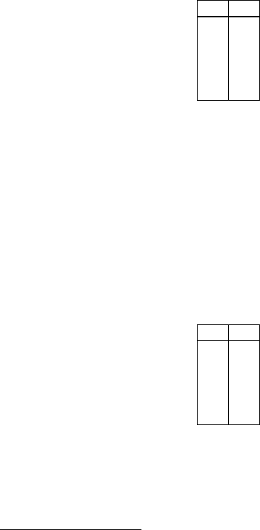
: The mean of this sample is

=(1.236,1.131)

and the covariance of

Table 1 Original sample values.

(1)

(2)

1.113 1.124

1.195 1.136

1.185 1.129

1.236 1.130

1.234 1.129

1.452 1.137

the sample is

V = 10

−3



11.01 0.343

0.343 0.020



, which may differ enough from

and V

to bias the stochastic program results. To correct for this problem, as long as K

is sufﬁciently large that

V has full rank, we can update the sample as follows to

produce a sample with mean

and covariance V :

0.5

(

−0.5

(

−

)), (3.3)

which results in the values in Table 10.3, which now has mean

and covariance V .

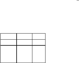
Table 2 Adjusted sample values.

1.044 1.116

1.118 1.148

1.109 1.127

1.155 1.127

1.153 1.125

1.351 1.137

These samples can then be used again to generate K

= 6 samples for period 2 (as-

suming serial independence). For a three period model, this results in K

= 36

total scenarios. Including a third set of realizations as in Section 1.2 would yield

Much larger samples are often used in practice for K

,but,since

t=1

grows quickly for

larger values of H , sample sizes for larger values of t are often small.

10.3 Scenario Generation and Distribution Fitting 429

= 216 scenarios, but often fewer scenarios are used in later periods. (In Exer-

cise 2, we use K

= 2 for 72 total scenarios.)

This procedure of modifying a random sample to match moments of an assumed

underlying distribution is called adjusted random sample generation. Results in

Kouwenberg [2001] suggest that this procedure can improve outcomes relative to

using random samples alone. Exercises 2 and 3 explore this issue for the ﬁnancial

planning example.

In addition to ﬁtting the mean and second moments, improved scenario trees

may result from ﬁtting higher moments, such as through ﬁts of skewness and kur-

tosis. Høyland and Wallace [2001] describe how to use an optimization procedure

to ﬁt these moments, which may include extreme values to represent tail risk and

inter-period moments to represent serial dependence. In experiments in Kouwenberg

[2001], the use of additional moment information provides minor improvement over

adjusting only for ﬁrst and second moments.

In longer horizon problems, an initial sampling procedure often still yields sce-

nario trees that are too large for efﬁcient direct computation. To simplify these trees

further, scenarios may be collapsed while retaining as much moment information

as possible (e.g., Cari˜no, et al. [1994]). Other alternatives in reducing scenario trees

are to ensure that the reduced tree stays as close as possible in a distribution metric

to the original (possibly sample-based) scenario tree (see Dupaˇcov´a, Gr¨owe, and

R¨omisch [2003]). Alternatively, a tree can be constructed directly that minimizes

the distance in the distribution metric to the original underlying distribution (Pﬂug

[2001]) or the tree can be adjusted (to be smaller or larger) in the process of so-

lution by examining the expected value of perfect information at each node of the

tree to collapse branches with small EVPI and to expand branches with large EVPI

(Dempster [2006]).

An important consideration for generating scenarios in ﬁnancial applications is,

unless conditions are known not to be in equilibrium, for the scenario trees not to

admit arbitrage in which trading among different assets could earn positive returns in

all scenarios without any initial investment. Arbitrage most often occurs in models

when derivative securities are included that depend on the same underlying security,

but their prices are not consistent with the set of scenarios.

Example 3

As an example, we again consider the ﬁnancial planning in Section 1.2 but with the

original two branches in each period and where short-selling (negative positions) of

the stock and bond are allowed. We now add an additional asset as a call option that

gives the holder of the option the right (but not the obligation) to buy the stock at

1.15 times its original price at the end of the ﬁrst period. In this way, the call option

has the following contingent payoff, C

, for each unit of stock value at time 0 ,

such that:

430 10 Multistage Approximations



0.10 if ξ

(1)=1.25,

0ifξ

(1)=1.10.

(3.4)

Suppose that the model includes a price for each unit of this call option of C

0.02 of the value of one unit of the stock. This would mean that the return value

(3) corresponding to the call option asset follows:

(3)=



5ifξ

(1)=1.25,

0ifξ

(1)=1.10.

(3.5)

Now, an initial investment strategy can include the following (x

(1),x

(2),x

(3)) =

(−18

,17

,1)

,forany

≥ 0 since this requires no additional wealth. The

wealth at the end of the ﬁrst period is then

(3)=



1.8067

=(−(18

)1.25 +(17

)1.14 + 5)

if ξ

(1)=1.25,

0ifξ

(1)=1.10,

(3.6)

which, as

→∞ , leads to inﬁnite wealth in the state where stocks increase in value

by 25%. The problem in this case is that C

= 0.02 is inconsistently low or ξ

(3)=

5 in the high-stock-value case is too high. Note that if instead ξ

(3)=3.1933 in

the high-stock-value scenario (corresponding to C

= 0.031524 ), then the wealth

is zero under both scenarios. This is the no-arbitrage condition that the future value

of a net initial investment of zero cannot be non-negative in all states and strictly

positive in some states (with probability greater than zero).

Consistent equilibrium prices (in a market with zero transaction costs and al-

lowable short sales) should satisfy the no-arbitrage condition; otherwise, investors

would exploit the price differences to create unlimited riskless proﬁts. To main-

tain this condition requires precise agreement of prices within a model. Transaction

costs, which are present to some degree in practice (for example, in the bid-ask

spread), allow for a range of consistent prices. Other restrictions, such as no-short-

sale constraints, can eliminate unbounded solutions in the model, but inconsistent

prices, even without pure arbitrage, can lead to solutions that are far from the op-

timal choice for a model with consistent prices. In the ﬁnancial planning example

considered here, for example, the optimal initial investment (Exercise 5) choices

are given in Table 3. The solution with the consistent high-stock-value return of

ξ(3)=3.1933 results in a balanced initial portfolio, while the solution of the model

using ξ(3)=5 for the high-stock-value scenarios places almost the entire portfolio

into the call option. Such wide swings can occur with small changes in the model

data from values consistent with equilibrium prices (see Exercise 5). Ensuring con-

sistent prices can then be a critical part of proper model generation.

The process we used to eliminate arbitrage can be simpliﬁed by using the equiv-

alent martingale measure or risk-neutral measure, i.e., a probability distribution

that weights scenarios based on their state prices to reﬂect a premium for non-

diversiﬁable risk such that the value of all ﬁnancial market assets equals the expected

value under this distribution of all future payoffs discounted by the risk-free rate

10.3 Scenario Generation and Distribution Fitting 431

(see Harrison and Kreps [1979]). Klaassen [1998] describes how this process ap-

plies for stochastic programming scenario trees, including important considerations

for maintaining consistency while aggregating states and periods as in Section 10.2.

Various methods can be used to represent the equivalent martingale measure by en-

suring consistency in the expectation and ﬁtting parameters to be consistent with

market prices. Alternatively, in some cases, it is possible instead to modify the con-

straints and to use the natural probability measure (again ensuring consistency) (see

Birge [2000]).

Theoretical results for obtaining convergence of solutions from a sample prob-

lem to that of the original problem are also possible for multistage problems as they

are for two-stage problems, but including adjustments such as matching moments

makes the analysis more difﬁcult and the theoretical bounds on convergence are of-

ten worse than what is actually observed. The basic multistage results are direct ex-

tensions of the two-period results. As shown in Shapiro [2003], under suitable con-

ditions (e.g., ﬁnite expecations, bounded sets of optimal solutions, and a pointwise

Strong Law of Large Numbers holding for the sample values, Q

t,K

) → Q

) ,

a.e.), then, as K

→ ∞,t = 1,...,H ,

• the sample average approximation value, z

→ z

∗

, the true optimal value;

• the distance between ﬁrst-stage optimal solution sets decreases to zero with

probability one;

• if the support of the true distribution is ﬁnite, then the ﬁrst-stage optimal solution

set is a nonempty face of the true optimal solution set with probability one.

For a special class of problems with non-negative objective values and non-negative

constraint matrices (except possibly in the ﬁrst and last stage), Swamy and Shmoys

[2005] show that, for any tolerance

> 0 , the required number of samples in a

multistage sample average approximation to achieve a high probability of a solution

within a 1 +

multiple of the optimal value is polynomial in

and a parameter

that depends on cost growth across time.

Table 3 Initial values of x

∗

for different returns on a call option.

ξ(3)= 3.1933 5.0

Asset

Stock 16.82 0.0

Bond 16.54 2.86

Call 21.64 52.14

432 10 Multistage Approximations

Exercises

1. Show that the assumption that logξ

∼ N(

) ,



0.141

0.122



and

−3



6.740 0.291

0.291 0.0784



matches the mean and variance of the stock and bond

returns for the ﬁnancial planning example in Section 1.2 and that the correlation

between the two assets is 0.4.

2. Solve the ﬁnancial planning example with a 72-scenario event tree correspond-

ing to two periods with returns given by

in Table 1 and one period with the

original two return realizations given in Chapter 1. Let the ﬁrst period solution

be ˆx

. Solve also for the 72-scenario event tree given by

in Table 2 and let

the ﬁrst period solution be ˜x

. To test for their relative performance of these

solution, perform a simulation with 1000 runs, where the initial allocations are

ˆx

and ˜x

respectively and the random returns are

for stage t drawn from

the underlying lognormal distribution. For each run k = 1,...,1000 , for the

second-period allocation, re-solve a two-stage model with input wealth (

)

ˆx

and (

)

˜x

respectively for the two alternatives and then obtain solutions on

the remaining (36-node) sample trees as ˆx

and ˜x

; then, use the second-

period return

, and repeat for the third and ﬁnal periods to obtain sample

objective values ˆz

and ˜z

. Compare the distributions of ˆz and ˜z for these

samples by plotting their percentiles. What does this suggest about the use of

adjusted samples?

3. Repeat Exercise 2 by randomly drawing ten additional random samples

and

adjusting to ﬁt the mean and covariance in

(so that now the tree has 2·16

512 scenarios). (Warning: this requires fast subproblem optimization.)

4. Suppose that instead of a call option to buy the stock at 15% above its current

value, the option is buy the stock at 10% above its current value. If this is in-

cluded in the ﬁnancial planning example with two branches per period, what

should the initial call price or premium C

be for this option to avoid arbitrage

possibilities?

5. Solve the 8-scenario, 3-period ﬁnancial planning example with the addition of

a call option. First, solve with the consistent high-stock-increase return on the

call option of 3.1933 and then with a high-stock-increase return of 5 . Verify

the solutions x

1∗

that are given in Table 3. Re-solve with ξ

(3)=3.20 in the

high-stock-return scenario. What is the value of initial investments x

1∗

now?

10.4 Multistage Sampling and Decomposition Methods

In this section, we consider algorithms that incorporate sampling into decomposition

methods for multistage stochastic programs with explicit conﬁdence intervals on

the convergence of the sample problem value to an optimal solution value. For the

10.4 Multistage Sampling and Decomposition Methods 433

exposition here, we consider multistage stochastic linear programs with relatively

complete recourse and a ﬁnite optimal objective value.

Assume that the stochastic elements are deﬁned over a discrete probability space

(

) ,P), where

⊗···⊗

is the support of the random data in stages

two through H , with

= {

=(h

(

),c

(

),T

t−1

·,1

(

),...,T

t−1

·,n

t−1

(

), i =

1,...,M

)}. Further, assume that the random parameters are serially independent.

Thus, the probability of a particular stage t realization

is constant from all pos-

sible (t −1) -stage scenarios.

For the following, we describe the strategy of abridged nested decomposition

(AND) (Donohue and Birge [2006]), which is an extension of the sampling strat-

egy of stochastic dual dynamic programming (SDDP) in Pereira and Pinto [1991].

Both algorithms use sampling to generate an upper bound on the expected value

(over an H -stage planning horizon) of a given ﬁrst stage solution and to use de-

composition to generate a lower bound. The algorithm terminates when the two

bounds are sufﬁciently close. As in the nested decomposition algorithm, each itera-

tion of SDDP and AND algorithm begins by solving the ﬁrst stage subproblem, after

which, KH-stage scenarios are sampled. Let x

and

denote the stage t solu-

tion vector and the stage t random parameter realization, respectively, in sampled

scenario k . A forward pass through a sampled version of the scenario tree solves the

nested decomposition subproblem (6.1.1–1.5) for stages t = 2,...,H and scenarios

k = 1,...,K .

The algorithm uses an upper bound estimate on z

∗

based on individual scenario

objective values, z

,where

= c

∑

t=2

(

, (4.1)

where x

is the same for all values of k .The z

values are combined to form an

estimate with K samples as:

ˆz

∑

k=1

, (4.2)

with standard deviation of the estimate given by,









∑

k=1

(ˆz

−z

)



. (4.3)

Using these values, a conﬁdence interval on the upper bound estimate can be con-

structed.

After the forward pass is completed, the method follows a backward pass as in

the nested decomposition algorithm, but, without considering all branches of the