Blank B.E., Krantz S.G. Calculus: Single Variable

Подождите немного. Документ загружается.

r 5

cðt Þdt

⁄ EX

AMPLE 5 A doctor injects 3 mg of dye into a vein near the patient’s

heart. The aortic concentration measurements have been tabulated, with time t

given in seconds and concentration c (t) given in milligrams per liter. Estimate the

patient’s cardiac output.

t 0

1 2345678

c(t) 0 0.54 2.7 6.6 8.9 6.4 3.1 1.2 0

Solution Because the partition has nine equally spaced points forming an even

number (N 5 8) of equal length subintervals, Simpson’s Rule is applicable:

cðt Þdt 

8 2 0

3  8

ð1ð0Þ1 4ð 0 :54Þ1 2ð2:7Þ1 4ð6:6Þ1 2ð8:9Þ1 4ð 6 :4Þ

1 2ð3:1Þ1 4ð1:2Þ1 1ð0ÞÞ

 29:453:

Therefore r is approximately 3/29.453 L/s, or 180/29.453 5 6.11 L/min.

INSIGHT

In Example 5, notice that the two data points equal to 0 have been

included in the sum just as they would have been had they had nonzero values. It is a

common error to omit data points that are 0 because they seem not to contribute to the

sum. In fact, each member of the sequence of data points, f (x

), f (x

),...

must be multiplied by the corresponding member of the sequence of coefﬁcients, 1, 4,

2, 4, . . . (in the case of Simpson’s Rule). Omitting an f (x

) that is 0 will lead to the

subsequent data points being multiplied by the wrong coefﬁcients.

QUICK QUIZ

1. Approximate

ð6=xÞdx by the Midpoint Rule with N 5 2.

2. Approximate

ð15=xÞdx by the Trapezoidal Rule with N 5 2.

3. Approximate

ð45=xÞdx by Simpson’s Rule with N 5 4.

4. Approximate

3:5

2:5

f ðxÞdx by a) the Midpoint Rule, b) the Trapezoidal Rule,

and c) Simpson’s Rule, using, in each case, as much of the data, f (2.5) 5 24,

f (3.0) 5 36, and f (3.5) 5 12, as possible.

Answers

1. 9 2. 28 3. 73 4. a) 36, b) 27, c) 30

EXERCISES

Problems for Practice

c In each of Exercises 1210, a function f, an interval I, and

an even integer N are given. Approximate the integral of f

over I by partitioning I into N equal length subintervals and

using the Midpoint Rule, the Trapezoidal Rule, and then

Simpson’s Rule. b

1. f ðxÞ5 x

I 5 ½1; 3; N 5 2

2. f ðxÞ5 x

1=2

I 5 ½0; 2; N 5 2

5.8 Numerical Techniques of Integration 455

3. f ðxÞ5

ﬃﬃﬃﬃﬃﬃﬃﬃﬃﬃﬃﬃﬃﬃﬃﬃﬃﬃﬃﬃﬃ

2 1 x 1 x

I 5 ½2 1; 1; N 5 2

4. f ðxÞ5 ð11x

ð1=3Þ

I 5 ½2 1; 1; N 5 2

5. f ðxÞ5 lnðxÞ I 5 ½1; 3; N 5 2

6. f ðxÞ5 15x=ð1 1 xÞ I 5 ½0; 4; N 5 4

7. f ðxÞ5 cosðxÞ I 5 ½π=4; 5π=4; N 5 4

8. f ðxÞ5

ﬃﬃﬃﬃﬃﬃﬃﬃﬃﬃﬃ

1 1 x

I 5 ½0; 8; N 5 4

9. f ðxÞ5 x

I 5 ½21=2; 7=2; N 5 4

10. f ðxÞ5 1=xI5 ½2; 6; N 5 4

c In each of Exercises 11214, a function f (x)

and an interval

I=[a, b] are given. Also given is the approximation M

A 5

f ðxÞdx that is obtained by using the Midpoint Rule

with a uniform partition of order 10.

a. Use

inequality (5.8.3) to ﬁnd a lower bound α for A.

b. Use inequality (5.8.3) to ﬁnd an upper bound β for A.

c. Calculate A and ascertain that it lies in the interval

[α, β]. b

11. f ðxÞ5 x 1 1=xI5 ½1=2; 7=2; M

5 7:93202:::

12. f ðxÞ5

ﬃﬃﬃﬃﬃﬃﬃﬃﬃﬃﬃ

1 1 x

I 5 ½0; 8; M

5 17:34205:::

13. f ðxÞ5 ð21xÞ

ð21=3Þ

I 5 ½2 1; 3; M

5 2:88409:::

14. f ðxÞ5 x

1 cosðxÞ I 5 ½0; π=2; M

5 2:28972:::

c In each of Exercises 15218, a function f (x)

and an interval

I 5 [a, b] are given. Also given is the approximation T

A 5

f ðxÞdx that is obtained by using the Trapezoidal Rule

with a uniform partition of order 10.

a. Use

inequality (5.8.6) to ﬁnd a lower bound α for A.

b. Use inequality (5.8.6) to ﬁnd an upper bound β for A.

c. Calculate A and ascertain that it lies in the interval

[α, β]. b

15. f ðxÞ5 x

I 5 ½25; 1; T

52158:160:::

16. f ðxÞ5 1=ð10 2 xÞ I 5 ½1; 8; T

5 1:51366:::

17. f ðxÞ5 xexpðx

Þ I 5 ½3=2; 2; T

5 22:64660:::

18. f ðxÞ5 secðxÞ I 5 ½0; π=4; T

5 0:88209:::

c In each of Exercises 19222, a function f (x)

and an interval

I=[a, b] are given. Also given is the approximation S

A 5

f ðxÞdx that is obtained by using Simpson’s Rule with

a uniform partition of order 10.

a. Use

inequality (5.8.8) to ﬁnd a lower bound α for A.

b. Use inequality (5.8.8) to ﬁnd an upper bound β for A.

c. Calculate A and ascertain that it lies in the interval

[α, β]. b

19. f ðxÞ5 x

I 5 ½1; 4; S

5 682:54050:::

20. f ðxÞ5 1=xI5 ½2; 10; S

5 1:61008:::

21. f ðxÞ5

ﬃﬃﬃﬃﬃﬃﬃ

ðxÞ

I 5 ½1; 9; S

5 17:33275:::

22. f ðxÞ5 10 sinðxÞ I 5 ½0; 3π=2; S

5 10:00281:::

c Income data for three countries are given in the following

tables.

In each table, x represents a percentage, and L(x) is

the corresponding value of the Lorenz function, as described

in Example 3. In each of Exercises 23227, use the speciﬁed

approximation

method to estimate the coefﬁcient of

inequality for the indicated country. (The values L (0) 5 0

and L (100) 5 100 are not included in the tables, but they

should be used.) b

x 20

40 60 80

L(x) 5203055

Income Data, Country A

x 25 50 75

L(x) 15 25 40

Income Data, Country B

x 10 20 30 40 50 60 70 80 90

L(x) 4 8 14 22 32 42 56 70 82

Income Data, Country C

23. Country A, Trapezoidal Rule

24. Country B, Trapezoidal Rule

25. Country C, Trapezoidal Rule

26. Country B, Simpson’s Rule

27. Country C, Simpson’s Rule

c In Exercises 28230, use Simpson’s Rule to estimate car-

diac

output based on the tabulated readings (with t in seconds

and c(t) in mg/L) taken after the injection of 5 mg of dye. b

28.

t 0

1.5 3 4.5 6 7.5 9

c(t) 0 2.4 6.3 9.7 7.1 2.3 0

29.

t 01 23 4 5 678

c(t) 0 1.9 5.8 9.4 10.4 9.1 5.9 2.1 0

30.

t 012345 67 8910

c(t) 0 3.8 6.8 8.6 9.7 10.2 9.4 8.2 6.1 3.1 0

Further Theory and Practice

31. Use inequality (5.8.6) to determine how large N should

be to ensure that the Trapezoidal Rule approximates

expð2x=2Þdx to within 10

? How about for Simpson’s

Rule?

c In each of Exercises 32235, a function f (x)

is given. Use

inequality (5.8.3) to determine how large N must be to guar-

antee that the Midpoint Rule approximation of

f ðxÞdx is

accurate to within 10

. b

456 Chapter

5 The Integral

32. f (x) 5 1/(3 1 x)

33. f ðxÞ5

ﬃﬃﬃﬃﬃﬃﬃﬃﬃﬃﬃ

6 1 x

34. f (x) 5 e

35. f (x) 5 sin(π x)

c In each of Exercises 36239, a function f (x)

is given. Use

inequality (5.8.8) to determine how large N must be to

guarantee that the Simpson’s Rule approximation of

f ðxÞdx is accurate to within 10

. b

36. f (x) 5 1/(3 1 x)

37. f ðxÞ5

ﬃﬃﬃﬃﬃﬃﬃﬃﬃﬃ

ﬃ

6 1 x

38. f (x) 5 e

39. f (x) 5 sin(π x)

40. Show that the Simpson’s Rule approximation is exact

when applied to a polynomial of degree 3 or less. (Hint:

Use inequality (5.8.4) to show that the error is 0.)

41. Show that the average of x

over the interval [γ2h, γ 1 h]

is γ (γ

1 h

). Show that this quantity is also equal to

((γ2h)

1 4 γ

1 (γ 1 h)

)/6. Deduce that Theorem 3,

which was stated for polynomials of degree 2, is also valid

for polynomials P (x) 5 Ax

1 Bx 1 C 1 Dx

of degree 3.

As a result, Simpson’s Rule is exact when applied to cubic

polynomials.

42. Applying Simpson’s Rule to the right side of

π 5 4

ﬃﬃﬃﬃﬃﬃﬃﬃﬃﬃﬃﬃﬃ

1 2 x

gives an approximation of π. In practice, this method of

approximation is not useful because of its computational

cost. For example, with N 5 100, the approximation is

3.1411 ..., which is accurate to only three decimal places.

Examine the graph of y 5

ﬃﬃﬃﬃﬃﬃﬃﬃﬃﬃﬃﬃﬃ

1 2 x

for 0 # x # 1. What

geometric property does this graph have that graphs of

approximating parabolas do not have? Why is error

bound (5.8.4) of no use here?

43. Simpson’s Rule is generally more accurate than the

Midpoint Rule, but it is not always more accurate. Cal-

culate A 5

ﬃﬃﬃﬃﬃ

jxj

dx. With N 5 2, estimate A using both

the Midpoint Rule, M

, and Simpson’s Rule, S

. What

are the absolute errors? Repeat with N 5 4.

44. Calculate A 5

jxjdx. Let N be an even positive integer

that is not divisible by 4. Show that if a uniform partition

of order N is used, then the Midpoint Rule approximation

of A is exact, but the Simpson’s Rule approximation is

not.

45. Suppose f has derivatives of order 4 in an interval con-

taining [a, b]. Chevilliet’s form of the error in Simpson’s

Rule states that the error in using Simpson’s Rule is exactly

ðb2 aÞ

180 N

ðf

000

ðξÞ2 f

000

ðηÞÞ

for two points ξ and η in [a, b]. Show that the error esti-

mate as stated in the text (sometimes known as Stirling’s

form) follows from Chevilliet’s form of the error.

c In Exercises 4

6 and 47, several values of the Lorenz func-

tion L have been tabulated (refer to Example 2). Use trape-

zoidal approximations to estimate the coefﬁcient of inequality

that corresponds to the given data. (Note: The tables represent

partitions that are not uniform. Also, the data points (0, 0) and

(100, 100) have not been included in the tables but should be

used in the calculations.) b

46.

x 15

25 50 75 90

L (x) 319254270

47.

x 16 28 51 75 88 97

L (x) 3 8 24 46 69 88

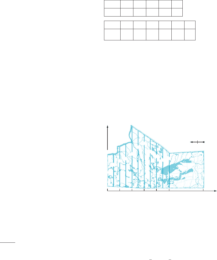
48. Figure 11 shows a map of the province of Manitoba

ﬂipped onto its western boundary. Distances are in kilo-

meters. The southern portion of the province, appearing

to the right in Figure 11, is essentially a trapezoid. Use

Simpson’s Rule to estimate the area of the northern

portion of the province. Approximately what is the area

of Manitoba when estimated in this way? (The actual area

is 649,953 km

.) Repeat with the Trapezoidal Rule.

Repeat with the Midpoint Rule using increments of 156 km

along the S-axis. (For more precise estimation, the small

arc of the eastern boundary that is not the graph of a

function must be taken into account.)

49. A 6 m wide swimming pool is illustrated in Figure 12, on

next page. Depths are given every 2 m. Estimate the

volume of water in the pool when it is ﬁlled. Use the

Midpoint, Trapezoidal, and Simpson’s Rules.

50. Let N be an even integer. The three approximation

methods discussed in this section satisfy

N=2

: ð5:8:9Þ

420

435

510

530

755

730

675

630

585

515

450

465

156 312 468 624

780

Distance

(

in kilometers

)

1225

MANITOBA

m Figure 11

5.8 Numerical Techniques of Integration 457

Use equation (5.8.9) to show that

ðS

2 T

N=2

Þ5 2 ðM

N=2

2 S

Þ:

c Let N be

an even integer. From equation (5.8.9) we may

deduce that one of the estimates T

N/2

and M

N/2

is greater

than or equal to S

, and the other is less than or equal to S

In each of Exercises 51254, calculate S

, M

N/2

, and T

N/2

for

the given even value of N and verify this deduction. b

51.

dx N 5 4

52.

ﬃﬃﬃ

dx N 5 2

53.

1=xdx N5 6

54.

sinðxÞdx N 5 4

55. During a 6-minute span, at intervals of 1 minute, the

speedometer of a car reads

Time (minutes) 0123456

Speed (km/hr) 90 80 75 80 80 70 60

Use Simpson’s Rule to estimate the distance traveled by

the car during that 6-minute period.

56. Speed measurements of a runner taken at half-second

intervals during the ﬁrst 5 seconds of a sprint are provided

in the following table.

About how many meters did the athlete run during that

5-second interval? Use Simpson’s Rule.

Calculator/Computer Exercises

c In each of Exercises 57260, a function f and an interval [a, b]

are speciﬁed. Plot y 5 jf

(x)j for a # x # b. Use your plot

and inequality (5.8.3) to determine the number N of sub-

intervals required to guarantee an absolute error no greater

than 5 3 10

when the Midpoint Rule is used to approximate

f ðxÞdx. State N and the resulting approximation. b

57. f ðxÞ5

ﬃﬃﬃﬃﬃﬃﬃﬃﬃﬃﬃﬃﬃﬃﬃﬃﬃﬃﬃﬃﬃﬃ

ﬃ

1 1 x 2

ﬃﬃﬃ

½1:25; 4

58. f ðxÞ5 x

ﬃﬃﬃﬃﬃﬃﬃﬃﬃﬃﬃﬃﬃ

1 1 x

½1=4; 4 

59. f (x) 5 sin(x)/x [1, 5]

60. f (x) 5 sin(x

) [1, 2]

c In each of Exercises 61264, a function f and

an interval

[a, b] are speciﬁed. Calculate the Simpson’s Rule approx-

imations of

f ðxÞdx with N 5 10 and N 5 20. If the ﬁrst ﬁve

decimal places do not agree, increment N by 10. Continue

until the ﬁrst ﬁve decimal places of two consecutive approx-

imations are the same. State your answer rounded to four

decimal places. b

61. f (x) 5 ln(1 1 x

) [0, 5]

62. f ðxÞ5 expð

ﬃﬃﬃ

Þ½1; 4

63. f ðxÞ5

ﬃﬃﬃﬃﬃﬃﬃﬃﬃﬃﬃﬃﬃ

1 1 x

½0; 4

64. f (x) 5 sin(π cos(x)) [0, π/3]

c In each of Exercises 65268, an integral

f ðxÞdx and a

positive integer N are given. Compute the exact value of the

integral, the Simpson’s Rule approximation of order N, and

the absolute error ε. Then ﬁnd a value c in the interval (a, b)

such that ε 5 (b2a)

(4)

(c)j/(180 N

). (This form of the error,

which resembles the Mean Value Theorem, implies inequal-

ity (5.8.4).) b

65.

ﬃﬃﬃ

dx N 5 6

66.

1=xdx N5 4

67.

ð11 xÞ

1=3

dx N 5 4

68.

ﬃﬃﬃﬃﬃﬃﬃﬃﬃﬃﬃ

1 1 x

dx N 5 4

69. Data is said to be normally distributed with mean μ and

standard deviation σ . 0 if, for every a , b, the probability

that a randomly selected data point lies in the interval [a, b]is

ﬃﬃﬃﬃﬃﬃ

2π

exp 2

x2μ





dx:

Suppose the scores on an exam are normally distributed

with mean 70 and standard deviation 15. Use Simpson’s

Rule with N 5 6 to approximate the probability that a

randomly selected exam has a grade in the range [ 55, 85].

(The answer, the probability of being within one standard

deviation of the mean, does not depend on the particular

values 15 and 70 of the parameters that are used in this

exercise.)

70. Suppose the scores on an exam are normally distributed

with mean 80 and standard deviation 10. (Refer to

Exercise 69.) What is the probability that a randomly

selected exam has a grade in the range [60, 100]? Use

3.9

0.77

1.5

2.0

2.4

2.8

3.1

3.4

3.6

m Figure 12

Time (s) 0 0.5 1.0 1.5 2.0 2.5 3.0 3.5 4.0 4.5 5.0

Speed (m/s) 0 5.26 6.67 7.41 8.33 8. 33 9.52 9.52 10.64 10.64 10.87

458 Chapter 5 The Integral

Simpson’s Rule with N 5 10. (The answer, the probability

of being within two standard deviations of the mean, does

not depend on the particular values 10 and 80 of the

parameters that are used in this exercise.)

71. The partition f0, 15, 25, 50, 75, 90, 100g of [0, 100] given in

Exercise 46 precludes an application of Simpson’s Rule

because it is not uniform. However, because the number

of subintervals is even, the idea behind Simpson’s Rule

can be used. Find the degree 2 polynomial p

that passes

through the three points (0, 0), (15, 3), and (25, 19). The

interpolation command of a computer algebra system will

make short work of ﬁnding this polynomial. Calculate

ðxÞdx. Next, ﬁnd the degree 2 polynomial p

that

passes through the three points (25, 19), (50, 25), and

(75, 42). Calculate

ðxÞdx. Repeat this procedure

with the last three points, (75, 42), (90, 75), and (100, 100).

What approximation of

100

LðxÞdx results?

72. The polynomial p

(x) of Exercise 71 is negative on the

subinterval (0, 11.42857 ...). As a result, the value of

11:42857:::

ðxÞdx underestimates

11:42857:::

LðxÞdx.To

compensate, averaging

ðxÞdx with the trapezoidal

approximation of

LðxÞdx, which is an overestimate,

might be considered. When the calculation of Exercise

71 is amended in this way, what approximation of

100

LðxÞdx results?

73. In a particular regional climate, the temperature varies

between 222



C and 40



C, averaging μ 5 11



C. The

number of days F (T) in the year on which the tempera-

ture remains below T degrees centigrade is given

(approximately) by

FðTÞ5

222

f ðxÞdx ð222 # T # 40Þ;

where

f ðxÞ5 12:72 exp



ðx2 11Þ

266:4



Notice that F (T) is the sort of area integral that we

studied in Section 5.4.

a. Use Simpson’s Rule with N 5 20 to approximate

F (40). What should the exact value of F (40) be?

b. Heat alerts are issued when the daily high temperature

is 36



C or more. On about how many days a year are

heat alerts issued?

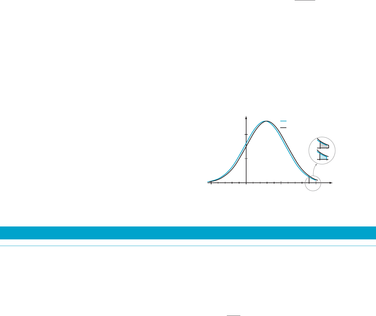
c. Suppose that global warming raises the average tem-

perature by 1



C, shifting the graph of f by 1 unit to the

right. The new model may be obtained by simply

replacing μ with 12 and using [221, 41] as the domain

(see Figure 13). What is the percentage increase in

heat alerts that will result from this 1



C shift in

temperature?

Summary of Key Topics in Chapter 5

Sigma Notation and

Partitions

(Sections 5.1, 5.2)

The notation

j5 M

means a

1 a

M11

1 a

M12

1 1 a

N21

1 a

The uniform partition of order N of an interval [ a, b] is the set fx

; x

;:::;x

of points x

deﬁned by

5 a 1 j 

b 2 a

ð0 # j # NÞ:

These points divide [a, b] into N subintervals, I

5 ½x

j21

; x

ð0 # j # NÞ.

Each subinterval has length Δx 5 ðb 2 aÞ=N.

shifted temperature

density

y  f(x)

20 0

20 40

m Figure 13

Summary of Key Topics 459

Area

(Section 5.1)

Let f be

a continuous positive function on [a, b]. The area of the region under the

graph of f, above the x-axis, and between the vertical lines x=a and x=b is the limit

as N tends to inﬁnity of the expression

j5 1

f ðx

ÞΔx

where Δx 5 ðb 2 aÞ= N and x

5 a 1 Δx; x

5 a 1 2Δx;:::; x

5 a 1 NΔx 5 b.

The Riemann Integral

(Section 5.2)

If f is

any function on an interval [a, b] that has been divided into N equal width

subintervals, and if for each j a points s

in the jth subinterval is chosen, then the

expression

Rðf ; S

Þ5

j5 1

f ðs

ÞΔx

is called a Riemann sum for f. Here we let S

denote fs

;: : : ;s

g. If the Riemann

sums for f have a limit as the number N of subintervals tends to inﬁnity, then that

limit is called the Riemann integral for f on [a, b], and f is said to be integrable on

[a, b]. The Riemann integral of f on [a, b] is denoted by

f ðxÞdx

and is said to be the deﬁnite integral of f over the interval [a, b]. A deﬁnite integral is

always a number. (By contrast, the indeﬁnite integral of f,

f ðxÞdx, denotes a

collection of functions of the variable of integration.)

Fundamental Theorem

of Calculus

(Sections 5.2 and 5.4)

A continuous function f is

integrable. The Fundamental Theorem of Calculus

consists of two formulas that relate differentiation and integration. Together they

imply that differentiation and integration are inverse operations. If f is continuous

on an interval I that contains the point a , then the function F de ﬁned on I by

FðxÞ5

f ðtÞdt;

is an antiderivative of f:

ðxÞ5 f ðx Þ:

If F is any antiderivative of f, then the deﬁnite integral of f can be calculated by

f ðxÞdx 5 FðbÞ2 FðaÞ:

Properties of the

Integral

(Section 5.3)

The integral satisﬁes the following ﬁve properties. If f and g are

integrable on [a, b]

and if α is a constant, then

ðf ðxÞ1 gðxÞÞdx 5

f ðxÞdx 1

gðxÞdx and

ðf ðxÞ2 gðxÞÞdx 5

f ðxÞdx 2

gðxÞdx;

αf ðxÞdx 5 α 

f ðxÞdx;

460 Chapter 5 The Integral

α dx 5 α ðb 2 aÞ;

f ðxÞdx 5 0; and

f ðxÞdx 1

f ðxÞdx 5

f ðxÞdx:

If b , a, then we deﬁne

f ðxÞdx to be equal to 2

f ðxÞdx.Iff is continuous on

[a, b], then the Mean Value Theorem for Integrals states that there is a c in (a, b)

such that

f ðcÞ5

b 2 a

f ðxÞdx:

Logarithmic and

Exponential Functions

(Section 5.5)

The natura

l logarithm can be deﬁned for positive x by

lnðxÞ5

dt:

All properties of the logarithm can be derived from this formula. The inverse of the

natural logarithm is called the natural exponential function,orexponential function

for short. It is denoted by exp. The number e is deﬁned by

e 5 exp ð1Þ:

If a is any positive number, and x is any real number, then we deﬁne

5 expðx lnðaÞÞ:

The familiar laws of exponents all follow from this deﬁnition.

Substitution

(Section 5.6)

If f (x)

has the form FðϕðxÞÞ ϕ

ðxÞ, then the calculation of the integral of f can be

simpliﬁed by a substitution of the form

u 5 ϕðxÞ and du 5 ϕ

ðxÞdx:

The Calculation of Area

(Section 5.7)

If f (x) $ 0o

n[a, b], then

f ðxÞdx

represents the area under the graph of f, above the x-axis, and between x 5 a and

x 5 b.Iff (x) # 0on[a, b], then the integral represents the negative of the area

above the graph of f, below the x-axis, and between x 5 a and x 5 b.

If f (x) $ g(x)on[a, b], then the area between the two graphs and between the

vertical lines x 5 a and x 5 b is given by

ðf ðxÞ2 g ðxÞÞdx:

To calculate the area between two graphs, it is necessary to break up the problem

into integrals over intervals on which one of the two functions is greater than or

equal to the other.

For some types of area problems, it is useful to integrat e in the y-variable,

treating x as the dependent variable.

Summary of Key Topics 461

Numerical Integration

(Section 5.8)

Methods of approximating deﬁnite integrals are particularly useful when an anti-

rivative of the integrand cannot be found. Let f be a continuous function on [a, b].

For a positive integer N, let Δx =(b 2 a)/N, x

5 a 1 jΔx, and x

5 ðx

j21

1 x

Þ=2. The

deﬁnite integral

f ðxÞdx can be approximated by the Midpoint Rule:

Δx ðf ð

Þ1 f ðx

Þ1 1 f ðx

ÞÞ:

The Trapezoidal Rule for approximating

f ðxÞdx is

Δx



f ðx

Þ1 2f ðx

Þ1 1 2f ðx

N21

Þ1 f ðx



Of these two methods of approximation, the Midpoint Rule is usually more accurate.

Still more accurate is Simpson’s Rule, which can be applied when N is even:

f ðxÞdx 

Δx



f ðx

Þ1 4f ðx

Þ1 2f ðx

Þ1 4f ðx

Þ1 1 2f ðx

N22

1 4f ðx

N21

Þ1 f ðx



For k 5 2 and k 5 4, let C

be a number such that the kth derivative f

(k)

satisﬁes

(k)

(x)| # C

on the interval [a, b] of integration. The errors that result from using

the Midpoint Rule, the Trapezoidal Rule, and Simpson’s Rule are no larger than



ðb 2 aÞ

;



ðb 2 aÞ

; and

180



ðb 2 aÞ

;

respectively.

REVIEW EXERCISES for Chapter 5

c In each of Exercises 124, use sigma notation to express

the sum. b

1. 1 1 4 1 9 1 16 1 

1 25

2. 120 1 122 1 124 1 126 1 1 240

3. 1=2 1 1=3 1 1=4 1 1=5 1 1=6 1 1 1=100

4. 1 2 2 1 3 2 4 1 5 2 6 1 2 100

c In each of Exercises 528, calculate the right endpoint

approximation of the area of the region that lies below the

graph of the given function f and above the given interval I of

the x-axis. Use the uniform partition of given order N. b

5. f ðxÞ5 x

I 5 ½2; 5; N 5 3

6. f ðxÞ5 1=xI5 ½1; 2; N 5 2

7. f ðxÞ5 ðx 2 1Þ=ðx 1 1Þ I 5 ½1; 4; N 5 3

8. f ðxÞ5 sinðxÞ I 5 ½0; π=2; N 5 3

c In each of Exercises 9212, for the given function f,

interval I,

and uniform partition of order N, evaluate the

Riemann sum Rðf ; SÞ using the choice of points S that con-

sists of the midpoints of the subintervals of I . b

9. f ðxÞ5 sinðxÞ; S 5 fπ=6; π=2g I 5 ½0; 2 π=3; N 5 2

10. f ðxÞ5 ð7 2 xÞ=x; S 5 f2; 4; 6g I 5 ½1; 7; N 5 3

11. f ðxÞ5 16 x

; S 5 f5=4; 7=4; 9=4; 11=4g I 5 ½1; 3; N 5 4

12. f ðxÞ5 x 2 x

; S 5 f1=8; 3=8; 5=8; 7=8g I 5 ½0; 1; N 5 4

c In each of Exercises 13228, evaluate the given deﬁnite

integral. b

13.

6 x

14.

ð10 x

1 9 x

Þdx

15.

ð1=xÞdx

16.

ﬃﬃﬃ

17.

ð2x 2 1=

ﬃﬃﬃ

Þdx

18.

π=3

π=6

sec

ðxÞdx

19.

π=3

π=6

ð4sinðxÞ2 cosðxÞÞdx

462 Chapter 5 The Integral

20.

π=4

secðxÞtanðxÞdx

21.

ð1=x

1=4

Þdx

22.

2=3

23.

ð24=x

Þdx

24.

lnð3Þ

25.

26.

π=2

π=4

csc

ðxÞdx

27.

π=2

π=4

cscðxÞcotðxÞdx

28.

ðx

1 x 1 2Þ=xdx

c In Exercises 29232, compute the average value of f over

[a, b],

and ﬁnd a point c in (a, b) at which f attains this

average value. b

29. f ðxÞ5 1=x

2=3

a 5 1; b 5 8

30. f ðxÞ5 x

a 5 1; b 5 5

31. f ðxÞ5

ﬃﬃﬃ

a 5 1; b 5 4

32. f ðxÞ5 1=x

a 5 1=2; b 5 3

In each of Exercises 33244 , a function F (x )anda

point c are given. Calculate F

(c). b

33. FðxÞ5

t 1 3

t 1 1

dt c 5 3

34. FðxÞ5

1=3

ﬃﬃﬃﬃﬃﬃﬃﬃﬃﬃﬃﬃﬃﬃ

ﬃﬃ

1 1

dt c 5 64

35. FðxÞ5

ðt

1 20Þ=ðt 1 2Þdt c 5 2

36. FðxÞ5

π=4

tan

ðtÞdt c 5 π=3

37. FðxÞ5

sin

ðπ=tÞdt c 5 4

38. FðxÞ5

ﬃﬃﬃﬃﬃﬃﬃﬃﬃﬃﬃﬃﬃﬃ

2 1

dt c 5 5

39. FðxÞ5

lnð1 1 tÞdt c 5 1

40. FðxÞ5

ﬃﬃﬃﬃﬃﬃﬃﬃﬃﬃﬃﬃﬃﬃ

1 1

ﬃﬃ

dt c 5 3

41. FðxÞ5

ðt

1t12Þ

2=3

dt c 5 1=3

42. FðxÞ5

t sinðtÞdt c 5 π=4

43. FðxÞ5

ﬃﬃﬃﬃﬃﬃﬃﬃﬃﬃﬃﬃ

5 1 t

dt c 5 2

44. FðxÞ5

ﬃﬃ

lnðtÞdt c 5 9

c In each of Exercises 45249 use the equations

ð1=tÞdt 5 3 and

ð1=tÞdt 5 6 to evaluate

ð1=tÞdt over

the given interval [a, b]. b

45. [1, αβ]

46. [1, β/α]

47. [α, β]

48. [α, αβ]

49. [1, α

]

c In each of Exercises 50270, make a substitution, and

evaluate

the given integral. b

50.

6xcosðx

Þdx

51.

cosðxÞ

sin

ðxÞ

52.

24 x

ﬃﬃﬃﬃﬃﬃﬃﬃﬃﬃﬃﬃﬃ

1 1 x

53.

24 x

ﬃﬃﬃﬃﬃﬃﬃﬃﬃﬃﬃﬃﬃ

2 1 x

54.

x 1 2

1 4x 1 5

55.

sinðxÞ

3 1 2cosðxÞ

56.

24sinð3xÞcos

ð3xÞdx

57.

ﬃﬃﬃ

11Þ

1=3

ﬃﬃﬃ

58.

2 π

cosðπ=x

59.

x ln

ðxÞ

60.



lnð2xÞ=x



61.

12 x

ﬃﬃﬃﬃﬃﬃﬃﬃﬃﬃﬃﬃﬃ

4x 1 1

62.

ðx11Þ

63.

ﬃﬃﬃﬃﬃﬃﬃﬃﬃﬃﬃ

x 1 2

64.

60 x

ﬃﬃﬃﬃﬃﬃﬃﬃﬃﬃﬃﬃﬃ

1 1

65.

arctan

ðxÞ

1 1 x

66.

expðxÞ

ﬃﬃﬃﬃﬃﬃﬃﬃﬃﬃﬃﬃﬃﬃﬃﬃﬃﬃﬃﬃﬃﬃ

1 1 expðxÞ

67.

arcsinðxÞ

ﬃﬃﬃﬃﬃﬃﬃﬃﬃﬃﬃﬃﬃ

1 2 x

68.

x 1 expð2xÞ

1 expð2xÞ

69.

1 2 2x

ﬃﬃﬃﬃﬃﬃﬃﬃﬃﬃﬃﬃﬃ

1 2 x

70.

2 1 x

4 1 x

c Evaluate the deﬁnite integrals in Exercises 71276. b

71.

π=9

24 tanð3xÞdx

72.

π=2

24 cotðx=3Þdx

73.

π=2

secðx=3Þdx

74.

exp ð4Þ

exp ð2Þ

x lnðxÞ

75.

ﬃﬃﬃﬃﬃﬃﬃﬃﬃﬃﬃﬃﬃ

9 1 x

76.

ﬃﬃﬃﬃﬃﬃﬃﬃﬃﬃﬃ

1 2 x

c In each of Exercises 77280, ﬁnd the area of the region that is

unded by the graphs of y 5 f (x)andy 5 g(x)forx between

the abscissas of the two point s of intersection. b

77. f ðxÞ5 4 2 x

gðxÞ5 3x

Review Exercises 463

78. f ðxÞ5 x

1 x 1 2 gðxÞ5 18 1 x 2 x

79. f ðxÞ52x

1 x

1 16 gðxÞ5 2x

2 2x

2 20

80. f ðxÞ5 2

gðxÞ5 1 1 2x 2 x

c In each of Exercises 81284, ﬁnd the total area of the

bounded regions whose upper and lower boundaries are arcs

of the graphs of the given functions f and g. b

81. f ðxÞ5 x

2 2x

2 3xgðxÞ5 0

82. f ðxÞ5 x

2 2x

1 3 gðxÞ5 1 1 x

83. f ðxÞ5 x

2 x

2 9x 1 4 gðxÞ525

84. f ðxÞ5 x

2 2x

1 1 gðxÞ5 1 2 x

c In each of Exercises 85288, a function f, an interval I, and

an even integer N are given. Approximate the integral of f

over I by partitioning I into N equal length subintervals and

using the Midpoint Rule, the Trapezoidal Rule, and then

Simpson’s Rule. b

85. f ðxÞ5 8 2 x

I 5 ½21; 3; N 5 2

86. f ðxÞ5 4x

1 1 I 5 ½1; 2; N 5 2

87. f ðxÞ5 ð 1 1 xÞ=ð1 1 4xÞ I 5 ½0; 2; N 5 4

88. f ðxÞ5 18x=ð1 1 8xÞ I 5 ½0; 1; N 5 4

c In each of Exercises 89292, a function f and

an interval

I 5 [a, b] are given. Also given is the approximation M

A 5

f ðxÞdx that is obtained by using the Midpoint Rule

with a uniform partition of order 10. Use the error estimate

for the Midpoint Rule approximation to ﬁnd a lower bound α

and and upper bound β for A. b

89. f ðxÞ5

ﬃﬃﬃﬃﬃﬃﬃﬃﬃﬃ

ﬃ

5 1 x

I 5 ½2 1; 11; M

5 37:34080:::

90. f ðxÞ5 x ð11xÞ

I 5 ½1; 3; M

5 138:08676:::

91. f ðxÞ5 ð 11xÞ

1=3

I 5 ½0; 7; M

5 11:25500:::

92. f ðxÞ5 lnð1 1 xÞ I 5 ½1; 6; M

5 7:23877:::

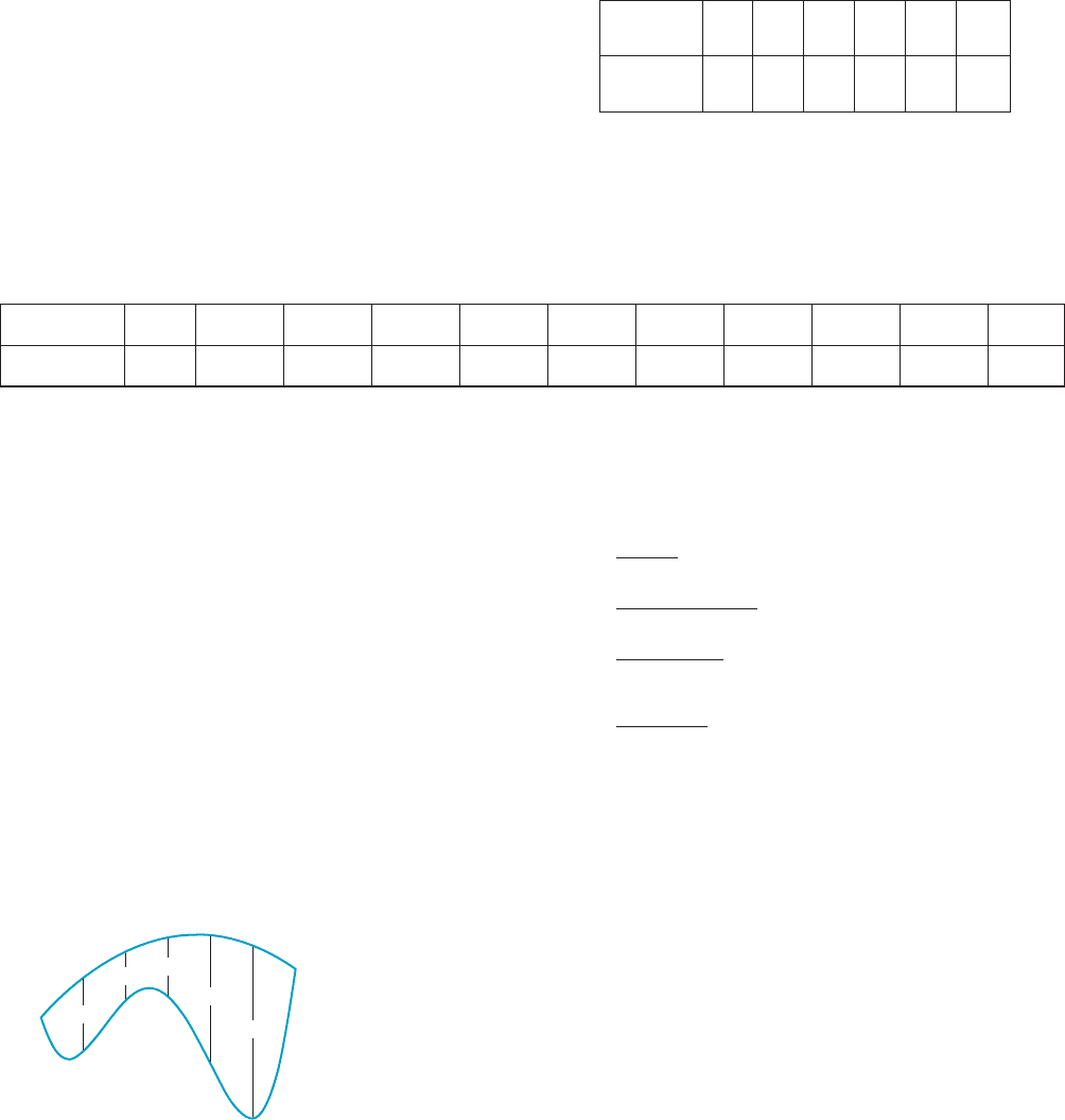
93. From west to east, a city is 5.1 km wide. North-south

measurements at 0.85 km intervals are given in Figure 1.

Use the Trapezoidal Rule and Simpson’s Rule to estimate

the city’s area.

94. During a 5-minute span, at intervals of 1 minute, the

speedometer of a car reads

Time

(minutes)

012345

Speed

(km/h)

80 74 60 54 46 0

Use the Trapezoidal Rule to estimate the distance tra-

veled by the car during that 5-minute period.

95. Speed measurements of a runner taken at half-second

intervals during the last 5 seconds of a sprint are provided

in the following table.

About how many meters did the athlete run during that 5-

second interval? Use Simpson’s Rule.

c In Exercises 96299, use a table of integrals to calculate the

given

integral. b

96.

ð11t

97.

ð2x 1 1Þðx13=2Þ

98.

36cosðtÞ



31sin

ðtÞ



99.

expð3tÞ

4 2 expð2tÞ

Time (s) 5.0 5.5 6.0 6.5 7.0 7.5 8.0 8.5 9.0 9.5 10.0

Speed (m/s) 10.66 10.69 10.86 10.98 10.96 10.94 10.80 10.71 10.64 10.58 10.43

8.67

5.79

7.02

15.22

20.46

m Figure 1

464 Chapter

5 The Integral