Caers J. Modeling Uncertainty in the Earth Sciences
Подождите немного. Документ загружается.


P1: OTA/XYZ P2: ABC
JWST061-04 JWST061-Caers March 29, 2011 9:9 Printer Name: Yet to Come
4.3 TOOLS FOR STRUCTURING DECISION PROBLEMS 71
recharge
at locaon 1
no
recharge
recharge
at locaon 2
(uncertain)
channel
orientaon
$ value 1
$ value 2
$ value 2
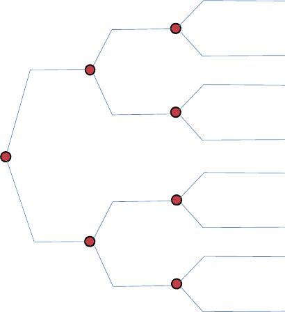
Figure 4.12 Elements of a decision tree.
Using these elements, trees are built from left to right, ordering the sequence of deci-
sions needed in function of time. An example decision tree for our recharge problem is
given in Figure 4.13. The first node represents the ultimate decision, that is, whether or
not to recharge and if so where to recharge. The subsequent decision is about whether
to choose a pond or a well if that choice is available. The uncertainty nodes are listed
after the decision node and may or may not be the same for each decision alternative. For
example, in location two there is no uncertainty about channel orientation as reflected in
the tree of Figure 4.13. We could also have included an additional decision as to whether
or not to recharge and then make a decision about location.
Much of this book will be devoted to assigning probabilities to uncertain events as well
as ways for calculating values of the end nodes. Indeed, in the example of Figure 4.13
a rather simplified situation is presented, since uncertainty about the Earth subsurface is
likely to be more complex than simply that of not knowing exactly channel orientation.
In this book, actual 3D Earth models will be built, and due to uncertainty one can build
many alternative models constrained to whatever data is available. These models allow
calculating responses due to engineering actions or decisions taken in reality such as the
NW
NE
NW
NE
NW
NE
Recharge
at locaon 1
no
Pond
Well
recharge
recharge
at locaon 2
Figure 4.13 Example of a decision tree.
P1: OTA/XYZ P2: ABC
JWST061-04 JWST061-Caers March 29, 2011 9:9 Printer Name: Yet to Come
72 CH 4 ENGINEERING THE EARTH: MAKING DECISIONS UNDER UNCERTAINTY
A:
orientaon
B:
thickness
C:
width
P(A=NW)
P(A=NE)
P(B=Low)
P(B=high)
P(B=Low)
P(B=high)
P(C=Low | B=low)
P(C=High | B=low)
P(C=Low | B=high)
P(C=high | B=high)
P(C=Low | B=low)
P(C=high | B=low)
P(C=Low | B=high)
P(C=high | B=high)
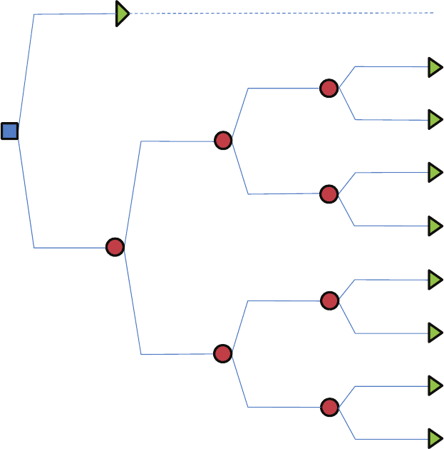
Figure 4.14 Example of hierarchies of uncertain variables in a tree.
decision to recharge or not. Flow simulators can be used to simulate the flow in the sub-
surface, thereby simulating the response of a recharge operation. Using economic model
calculations, the output of these simulators can then be used to assign a value to each
node, for example in this case based on the salt concentration of pumping groundwater
out of the aquifer and how that will affect the growth of crops. At this point we will not
deal with constructing decision trees when multiple alternative models are the specific
representation of uncertainty, for this refer to the chapter on Value of Information.
In simpler cases where uncertainty is simply about a few variables, the decision tree
should reflect the mutual dependence between several variables. For example, if, in ad-
dition to channel orientation, channel thickness and width is uncertain, then it can be as-
sumed from sedimentological arguments that width and thickness are dependent variables
but independent of channel orientation. Recall from Chapter 2 that dependency between
random variables is modeled through conditional probabilities and that if two variables
A and B are independent then P(A|B) = P(A). Figure 4.14 sketches a plausible situation
for the case with channel orientation, thickness and width. Note how some probabilities
are conditional while others are not, reflecting the nature of dependency between these
various variables.
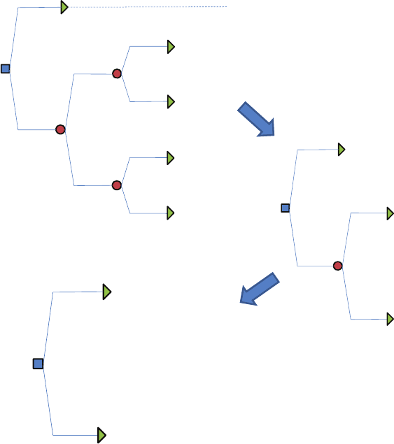
4.3.3 Solving Decision Trees
Solving a decision tree entails determining the optimal decision for the leftmost (i.e.,
ultimate) decision by maximizing an expected value. To achieve this, the tree is solved
from right to left using the following method:
P1: OTA/XYZ P2: ABC
JWST061-04 JWST061-Caers March 29, 2011 9:9 Printer Name: Yet to Come
4.3 TOOLS FOR STRUCTURING DECISION PROBLEMS 73
1 Select a rightmost node that has no successors.
2 Determine the expected payoff associated with the node:
a If it is a decision node: select the decision with highest expected value
b If it is a chance node: calculate its expected value.
3 Replace the node with its expected value.
4 Go back to step 1 and continue until you arrive at the first decision node.
Consider the drinking water contamination example introduced at the beginning of
the chapter. Figure 4.15 shows the decision tree which can be read from left to right as
follows: the decision is whether to clean up or not, in case of a clean up decision, the gov-
ernment needs to pay the cost, which is $15 million (hence a value of −15). In case of a
channels
sand bars
Orientaon = 150
Orientaon = 50
Orientaon = 150
Orientaon = 50
connected
not connected
connected
not connected
connected
not connected
connected
not connected
–15 cost of clean up
–50 cost of law suit
0 No cost
–50 cost of law suit
0 No cost
–50 cost of law suit
0 No cost
–50 cost of law suit
0 No cost
0.5
0.5
0.4
0.6
0.4
0.6
0.89
0.11
0.55
0.45
0.41
0.59
0.02
0.98
Clean
Do not clean
Figure 4.15 Decision tree for the groundwater contamination problem (red are probabilities for
that node).
P1: OTA/XYZ P2: ABC
JWST061-04 JWST061-Caers March 29, 2011 9:9 Printer Name: Yet to Come
74 CH 4 ENGINEERING THE EARTH: MAKING DECISIONS UNDER UNCERTAINTY
decision to not clean up the site, there is a potential for a law suit. This is subject to chance
because the law suit will only happen when the drinking water is polluted, which in turn
will happen when the geology of the subsurface is unfavorable. Such an “unfavorable”
situation occurs when a subsurface “connection” exists between the contaminant source
and the well. A connection means that there is a path through which contaminants can
travel from one point to another. In subsequent chapters, how to calculate the probability
of such connection occurring given the geological uncertainty is discussed. For now,
assume two scenarios, “connected” and “not-connected,” and assume the probability for
all possible cases of geological uncertainty is known. Such uncertainty presents itself
at two levels (and they are assumed to be hierarchical, so the order in the tree matters):
uncertainty in geological scenario (presence of channels vs presence of bars) and
uncertainty in orientation for a given geological scenario, both being binary and discrete.
The cost of the law suit is set at $50 million (although this is usually uncertain as well).
Starting now from right to left, the tree is “solved” by calculating the expected values
for each branch (Figure 4.16) until the decision node is reached. The optimal decision is
then to clean up, since this has the smallest cost (largest value).
channels
sand bars
Orientaon = 150
Orientaon = 50
Orientaon = 150
Orientaon = 50
–15 cost of clean up
0.5
0.5
0.4
0.6
0.4
0.6
Clean
Do not clean
–44.5 = –0.89×50 + 0.11×0
–27.5
–20.5
-1
channels
sand bars
–15 cost of clean up
0.5
0.5
Clean
Do not clean
–34.3 = –0.4×44.5 – 0.6×27.5
–8.6 = –0.4×20 – 0.6×1
–15 cost of clean up
Clean
Do not clean
–21.5 = –0.5×34.3 – 0.5×8.6
Figure 4.16 Solving the decision tree from right to left for the groundwater contamination
problem.
P1: OTA/XYZ P2: ABC
JWST061-04 JWST061-Caers March 29, 2011 9:9 Printer Name: Yet to Come
4.3 TOOLS FOR STRUCTURING DECISION PROBLEMS 75
0
10
20
30
40
120100806040200
Cost of Clean Up/No Clean Up
Cost of Law Suit
Cost of No Clean Up
Cost of Clean Up
0
10
20
30
10.750.50.250
Cost of Clean Up/No Clean Up
Probability of Channel Deposional Model
Cost of No Clean Up
Cost of Clean Up
clean
Do not clean
clean
Do not clean
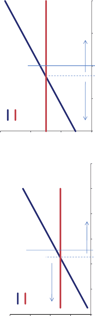
Figure 4.17 Sensitivity of the decision made for (left) changing the cost of law suit and (right) the probability associated with the channel
depositional model.
P1: OTA/XYZ P2: ABC
JWST061-04 JWST061-Caers March 29, 2011 9:9 Printer Name: Yet to Come
76 CH 4 ENGINEERING THE EARTH: MAKING DECISIONS UNDER UNCERTAINTY
4.3.4 Sensitivity Analysis
As discussed previously, establishing absolute values, such as the expected values cal-
culated in a tree, is less important than figuring out what has the most impact on these
values. This is the goal of a sensitivity analysis. The decision emanating from solving a
given decision tree such as the one in Figure 4.15 depends on the probabilities associated
with uncertain events and the costs/payoffs of the end-nodes. Often, prior probabilities
such as the probability stated on each geological scenario (channel or bars) emanate from
expert judgments rather than from an actual frequency calculation (Chapter 2). Figuring
out whether the decision is strongly dependent on such probabilities will provide some
confidence (or possibly lack thereof) on the actual decision made. Figure 4.17 shows an
example of varying the probability associated with the depositional model, if a 50/50
chance for channel and bars is taken as the base case. The decision would change if the
channel probability changes to 0.42, which is not a large change, so putting some extra
effort on these prior probabilities by interviewing several experts may be worth the effort.
In another example, the cost of the law suit (base case = $50 million) can be varied.
The decision would change when the law suit cost drops to around $46 million, hence
only a small change is required. Any information that could impact these numbers may
therefore be valuable to the decision process. This concept of change due to collecting or
using more data is elaborated on in Chapter 11, termed “the value of information.”
Further Reading
Bratvold, R. and Begg S. (2010) Making Good Decisions, Society of Petroleum Engineers, Austin, TX.
Clemen, R.T. and Reilly, T. (2001) Making Hard Decisions, Duxbury, Pacific Grove, CA.
Howard, R.A. (1966) Decision analysis: applied decision theory, in Proceedings of the Fourth Interna-
tional Conference on Operational Research (eds D.B. Hertz and J. Melese), John Wiley & Sons, Inc.,
New York, NY, pp. 55–71.
Howard, R.A. and Matheson, J.E. (eds) (1989) The Principles and Applications of Decision Analysis,
Strategic Decisions Group, Menlo Park, CA.
McNamee, P. and Celona, J. (2005) Decision Analysis for the Professional, 4th edn, SmartOrg, Inc.,
Menlo Park, CA.
P1: OTA/XYZ P2: ABC
JWST061-05 JWST061-Caers March 29, 2011 9:6 Printer Name: Yet to Come
5
Modeling Spatial Continuity
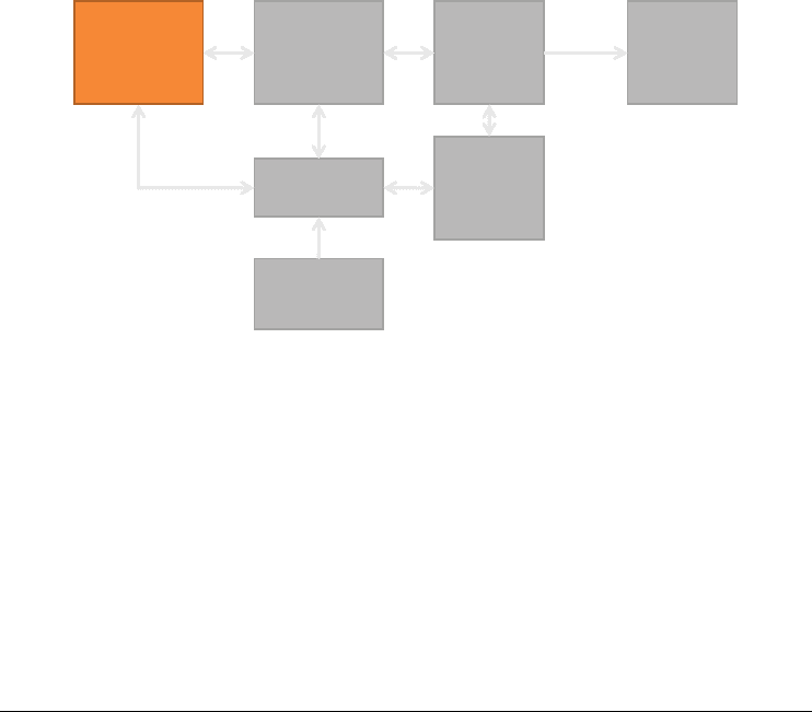
Modeling spatial continuity is critical to the question of addressing uncertainty, since a spa-
tial model of the properties being studied will lead to a different assessment of uncertainty
compared to assuming everything is random.
Physical
model
Spaal
Stochasc
model
Spaal
Input
parameters
Forecast
and
decision
model
Physical
input
parameters
Raw
observaons
Data sets
response
uncertain
uncertain
certain or uncertainuncertain
uncertain/error
uncertain
uncertain
5.1 Introduction
Variability in the Earth Sciences manifests itself at many levels: properties vary in space
and/or time with alternating high and low values. The spatial distribution, that is, the
characteristics of how these highs and lows vary is important for many engineering and
decision making problems. Mathematical models are needed to characterize this spatial
distribution then create Earth models (i.e., assign properties to a grid) that reflect the con-
ceptualized spatial distribution. However, due to incomplete information this conceptual
model is subject to uncertainty. Moreover, a mathematical model or concept can only
partially capture true variability.
Modeling Uncertainty in the Earth Sciences, First Edition. Jef Caers.
© 2011 John Wiley & Sons, Ltd. Published 2011 by John Wiley & Sons, Ltd.
77
P1: OTA/XYZ P2: ABC
JWST061-05 JWST061-Caers March 29, 2011 9:6 Printer Name: Yet to Come
78 CH 5 MODELING SPATIAL CONTINUITY
The non-randomness of Earth Sciences phenomena entails that values measured close
to each other are more “alike” than values measured further apart, in other words a spa-
tial relationship exists between such values. The term “spatial relationship” incorporates
all sorts of relationships, such as relationships among the available spatial data or be-
tween the unknown values and the measured data. The data may be of any type, pos-
sibly different from that of the variable or property being modeled. Therefore, in order
to quantify uncertainty about an unsampled value, it is important to first and foremost
quantify that spatial relationship, that is, quantify through a mathematical model the un-
derlying spatial continuity. In this book such a model is termed a “spatial continuity
model”. The simplest possible quantification consists of evaluating the correlation coef-
ficient between any datum value measured at locations u = (x,y,z) and any other mea-
sured a distance h away. Providing this correlation for various distances h will lead to
the definition of a correlogram or variogram, which is one particular spatial continuity
model discussed.
In the particular case of modeling the subsurface, spatial continuity is often determined
by two major components: one is the structural features such as fault and a horizon sur-
faces; the second is the continuity of the properties being studied within these structures.
Since these two components present themselves so differently, the modeling of spatial
continuity for each is approached differently, although it should be understood that there
may be techniques that apply to both structure and properties. Modeling of structures is
treated in Chapter 8.
In terms of properties, this chapter presents various alternative spatial continuity
models for quantifying the continuity of properties whether discrete or continuous and
whether they vary in space and or time. This book deals mostly with spatial processes
though, understanding that many of the principles for modeling spatial processes apply
also to time processes or spatio-temporal processes (both space and time). The models
developed here are stochastic models (as opposed to physical models) and are used to
model so-called “static” properties such as a rock property or a soil type. They are rarely
used to model dynamic properties (those that follow physical laws) such as pressure or
temperature, unless it is required to interpolate pressure and temperature on a grid or do a
simple filtering operation or statistical manipulation. Dynamic properties follow physical
laws and their role in modeling uncertainty is the topic of Chapter 10.
Three spatial models are presented in this chapter: (i) the correlogram/variogram
model, (ii) the object (Boolean) model, and (iii) the 3D training image models. As
with any mathematical model, “parameters” are required for such models to be com-
pletely specified. The variogram is a model that is built based on mathematical consid-
erations rather than physical ones. While the variogram may be the simplest model of
the set, requiring only a few parameters, it may not be easy to interpret from data when
there are few, nor can it deliver the complexity of real spatially varying phenomena. Both
the object-based and the training image-based models attempt to provide models from
a more realistic perspective, but call for a prior thorough understanding and interpreta-
tion of the spatial phenomenon and require many more parameters. Such interpretation is
subject to a great deal of uncertainty (if not one of the most important one).
P1: OTA/XYZ P2: ABC
JWST061-05 JWST061-Caers March 29, 2011 9:6 Printer Name: Yet to Come
5.2 THE VARIOGRAM 79
5.2 The Variogram
5.2.1 Autocorrelation in 1D
The observation that is made at a certain time instant t
i
is generally not independent
from the time observation at, for example, the next time instant t
i + 1
. Or, in space, the
observation made at a position x
i
is not independent of the observation made at a slightly
different position x
i + 1
. For prediction purposes, it is often very important to know how
far the correlation or association extends or what the exact nature of this association
is. We would like to design a measure of association for each time or space interval. We
expect that, for small time intervals, the two events separated by this interval are very well
associated. However, as the time interval increases, we expect the association to decrease.
In Chapter 2 a measure of linear association between two variables X and Y, namely the
correlation coefficient, was defined. Here, this idea is extended to one variable measured
at different instances in time. Recall the equation for the correlation between X and Y:
r =
1
n − 1
n
i=1
x
i
− x
s
x
·
y
i
− y
s
y
The correlation measured between two variables X and Y is applied to the correlation
measured between the same variable Y but measured at different time instances. We will
consider time instances that are t apart.
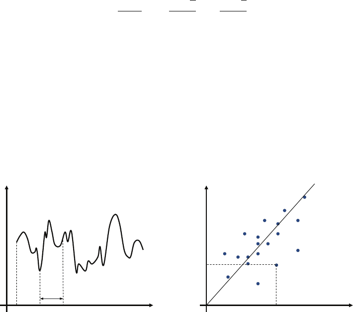
Using a sliding scheme (Figure 5.1), the pair [Y(t),Y(t + t)] are moved over the
time axis, each time t, recording the values of y(t) and y(t + t). The pair [y(t), y(t +
t)] represents one single point in the scatter plot of Figure 5.1. n(t) is the number of
pairs of data found by applying this slide rule for a given t. It is observed that as t
increases, fewer data pairs are found simply because the time series has a limited record.
The complete scatter plot in Figure 5.1 is then used to calculate the correlation coefficient
t
t + Δt
tme
Y(t) "signal", "reponse", "measurement"
t lag distanceΔ
scaer plot for tΔ
y(t)
y(t + Δt)
Figure 5.1 A 1D time series (left). Calculating the correlation coefficient for a given lag distance
or time interval t (right).
P1: OTA/XYZ P2: ABC
JWST061-05 JWST061-Caers March 29, 2011 9:6 Printer Name: Yet to Come
80 CH 5 MODELING SPATIAL CONTINUITY
for that value of t. Calculating the correlation coefficient for various intervals t and
plotting r(t) versus t results in the correlogram or autocorrelation plot.
What does the autocorrelation plot measure?
r
When t = 0: the value r = 1 is retained. Indeed, y(t) is perfectly correlated with itself.
r
When t > 0: One expects the correlation r to become smaller. Indeed, events that are
farther spread apart in time or space are less correlated with each other.
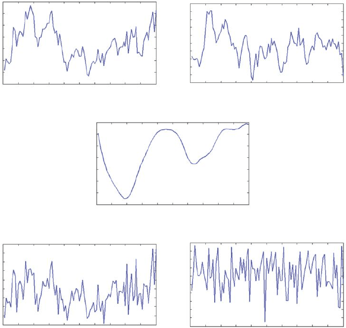
A few simple example cases are shown in Figure 5.2a and 5.2b. In Case 1, it can
be observed how the correlation coefficient becomes approximately zero at twenty time
1.5
Case 1 Case 2
Case 3
Case 4 Case 5
1
0.5
0
-0.5
-1
-1.5
-2
0 1020304050
Time t
60 70 80 90 100
Y(t)
1.5
2
2.5
3
1
0.5
0
-0.5
-1
-1.5
-2
0 1020304050
Time t
60 70 80 90 100
Y(t)
2
1.5
2.5
1
0.5
0
-0.5
-1
-1.5
-2
0 1020304050
Time t
60 70 80 90 100
Y(t)
1
0.5
0
-0.5
-1
-1.5
-2
-2.5
0 1020304050
Time t
60 70 80 90 100
Y(t)
1.5
2
1
0.5
0
-0.5
-1
-1.5
-2
-2.5
-3
0
(a)
10 20 30 40 50
Time t
60 70 80 90 100
Y(t)
Figure 5.2 (a) Example time series; (b) correlograms corresponding to the time series.