Caers J. Modeling Uncertainty in the Earth Sciences

Подождите немного. Документ загружается.

P1: OTA/XYZ P2: ABC

JWST061-05 JWST061-Caers March 29, 2011 9:6 Printer Name: Yet to Come

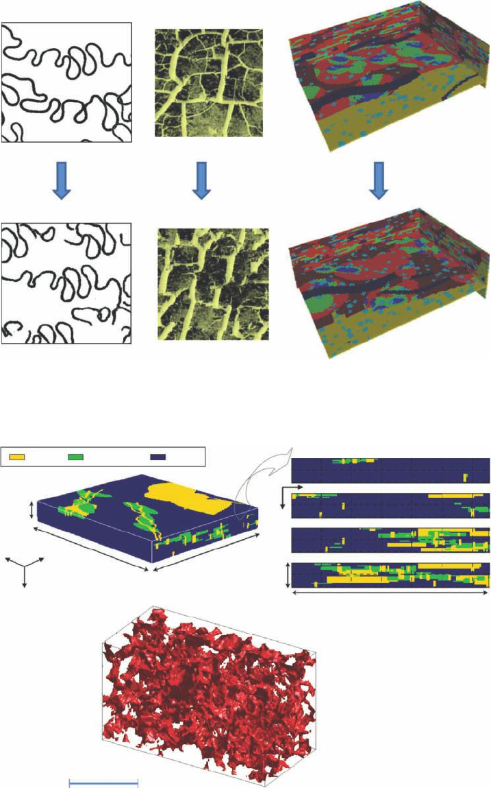
Training images

Earth models mimicking the training image paerns

Figure 5.11 A few example training images and Earth models produced from them exhibiting

similar patterns.

sand

112 (m)

15 (km)

13 (km)

overbank shale

112 (km)

microns

13 (km)

Figure 5.12 3D Training image example at the basin scale and pore scale (red = pore space).

P1: OTA/XYZ P2: ABC

JWST061-05 JWST061-Caers March 29, 2011 9:6 Printer Name: Yet to Come

92 CH 5 MODELING SPATIAL CONTINUITY

Further Reading

Caers, J. and Zhang, T. (2004) Multiple-point geostatistics: a quantitative vehicle for integrating geologic

analogs into multiple reservoir models, in Integration of outcrop and modern analog data in reservoir

models (eds G.M. Grammer, P.M. Harris and G.P. Eberli), AAPG Memoir 80, American Association

of Petroleum Geologists, Tulsa, OK, 383–394.

Deutsch, C.V. and Journel, A.G. (1998) GSLIB: The Geostatistical Software Library, Oxford University

Press.

Halderson, H.H. and Damsleth, E. (1990) Stochastic modeling. Journal of Petroleum Technology, 42(4),

404–412.

Holden, L., Hauge, R., Skare, Ø., and Skorstad, A. (1998) Modeling of ﬂuvial reservoirs with object

models. Mathematical Geology, 30, 473–496.

Isaaks, E.H. and Srivastava, R.M. (1989) An introduction to applied geostatistics, Oxford University

Press.

Ripley, B.D. (2004) Spatial statistics, John Wiley & Sons, Inc., New York.

P1: OTA/XYZ P2: ABC

JWST061-06 JWST061-Caers March 30, 2011 19:10 Printer Name: Yet to Come

Modeling Spatial Uncertainty

The set of models that can be generated for a given (ﬁxed) spatial continuity model represents

a type of uncertainty that is termed spatial uncertainty or model of spatial uncertainty. It is

important to recognize that this is only one component in the large model of uncertainty that

is being built in this book.

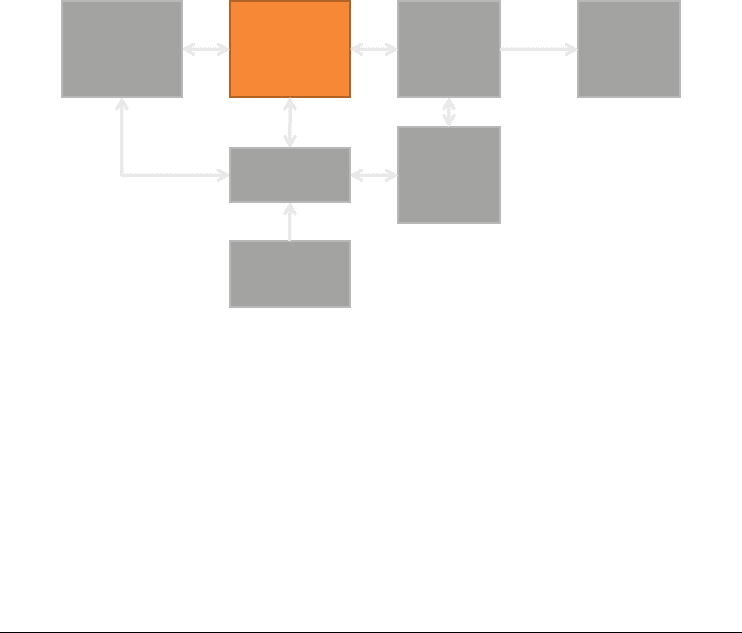
Physical

model

Spaal

Stochasc

model

Spaal

Input

parameters

Forecast

and

decision

model

Physical

input

parameters

Raw

observaons

Data sets

response

uncertain

uncertain certain or uncertain

uncertain/error

uncertain

6.1 Introduction

A variogram model, Boolean model or 3D training image provides a model for the spatial

continuity of the phenomenon being studied. This was the topic of the previous chapter.

In this chapter methods for generating an Earth model that reﬂects what is captured in

this spatial continuity model are discussed. Recall that an Earth model is simply a 3D

grid ﬁlled with one or more properties. It will be seen that this creation is not a unique

process; many Earth models that are reﬂective of the same spatial continuity can be cre-

ated. The set of models that can be generated for a given (ﬁxed) spatial continuity model

Modeling Uncertainty in the Earth Sciences, First Edition. Jef Caers.

P1: OTA/XYZ P2: ABC

JWST061-06 JWST061-Caers March 30, 2011 19:10 Printer Name: Yet to Come

94 CH 6 MODELING SPATIAL UNCERTAINTY

represents a type of uncertainty that is termed spatial uncertainty or model of spatial un-

certainty. It is important to recognize that this is only one component in the large model

of uncertainty that is being built in this book. If conceptually the Earth is understood

as inﬁnitely long one-dimensional layers, then only one model can be created: a layered

model. If channel-type structures are assumed to exist and modeled in a Boolean model,

then there are many ways to spatially distribute these channels in 3D space in a way that

is geologically realistic following the geological rules speciﬁed by the Boolean model. In

this chapter various techniques to accomplish this are discussed, then, in the next chapter,

it is shown how this spatial uncertainty can be further constrained with various sources

of data.

6.2 Object-Based Simulation

As discussed previously, object models allow the shape of objects occurring in nature to

be realistically represented. The aim of an object-based algorithm is to generate multi-

ple Earth models by dropping onto the grid objects in such a way that they ﬁt the data.

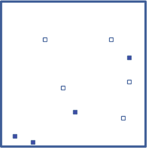
For now only one data source is considered: point observations. These are simply ob-

servations (of a certain volume or support) that are assumed to be of the same size as

the model grid cell and are direct observations of the phenomenon. In this case, we have

observations of the object type at speciﬁc locations (Figure 6.1).

Object-based models are evidently more “rigid” than cell-based, since “morphing” a

set of objects into a model constrained to all data is not as trivial as changing a few indi-

vidual grid cells to achieve the same task. This is particularly true for large, continuous

objects such as sinuous channels. The existing software implementations therefore rely

on an iterative approach to constrain such models to data. A trial-and-error procedure

is required to obtain models that reﬂect correctly the Boolean model and to adequately

match data. Boolean Earth models that are not constrained to any data locally can be

generated; this is called in geostatistical jargon “unconditional simulation.”

Figure 6.1 Point data with two categories.

P1: OTA/XYZ P2: ABC

JWST061-06 JWST061-Caers March 30, 2011 19:10 Printer Name: Yet to Come

6.2 OBJECT-BASED SIMULATION 95

For unconditional Boolean simulation with one object type, an Earth model can be

simply simulated without iteration by placing the objects randomly in the Earth model

grid and continuing until the desired proportion of objects is achieved. However, when

multiple interacting objects need to be placed in the same grid or when the placement

of objects need to follow certain rules, it is often necessary to “iterate,” for example by

moving the objects around until the rules expressed in the Boolean model are respected.

Iteration is required since it would be too hard to achieve this by a stroke of luck in

the ﬁrst iteration. The same holds when there are data that need to be matched. These

iterative approaches start by generating an initial model that follows the pre-deﬁned shape

description but does not necessarily ﬁt the local data or follow all the rules. The most

critical part in making the iterative approach successful is the way in which a new object

model is generated, perturbed from the initial or current one. The type of perturbation

performed will determine how efﬁcient the iterative process is, how well the ﬁnal object

model matches the data and how well the pre-deﬁned parameterization of object shapes

is maintained. One iteration step in this iterative scheme consists of:

proposing a perturbation of the current 3D Earth model;

accepting this perturbation with a certain probability ␣: this means that there is some

chance, namely 1 − ␣, that a model perturbation that improves the data matching will

be rejected. This is needed in order to cover as much as possible all possible spatial

conﬁgurations of objects that match equally well the data.

Several theories on so-called Markov chains (a process whereby the next iteration

accounts only for the previous one) have been developed on deﬁning the optimal pertur-

bation and on determining the probability ␣ at each iteration step and are speciﬁc to the

type of objects present. These are not discussed in this book, as this is more advanced ma-

terial. Importing objects and arbitrarily morphing them to match the data could be done

easily. But then odd or unrealistic shapes may be generated. The key lies in determining

values for ␣ that achieve two goals: (1) matching data and (2) reﬂecting the predeﬁned

Boolean model.

Regardless of the numerous smart implementations, the most challenging obstacle in

using object-based algorithms lies in the mismatch between the object parameterization

and the actual data. Some discrepancy exists between the simpliﬁed geometrical shapes

and actual occurrence in nature; reducing that discrepancy may call for considerable CPU

demand due to long iterations. It is often not possible to predict the level of discrepancy

prior to starting the object-based algorithms. While the object-based approach is a general

approach in the sense that any type of object could be modeled, the iterative approaches

to constraining such models to data are usually object speciﬁc.

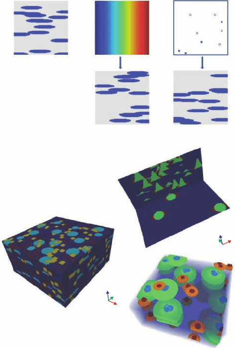
A few examples of typical rules and geometries used on object simulation are shown

in Figure 6.2. Case 1 has a simple elliptical object randomly distributed with a proportion

of 30%. Case 2 shows the same elliptical object, but having a proportion that varies in

space according to the map shown in Figure 6.2 (red color meaning higher proportion).

Case 3 shows an Earth model constrained to the data of Figure 6.1. Case 3 shows

P1: OTA/XYZ P2: ABC

JWST061-06 JWST061-Caers March 30, 2011 19:10 Printer Name: Yet to Come

96 CH 6 MODELING SPATIAL UNCERTAINTY

Cas

Case 2 Case 3

Cas

Figure 6.2 A few example cases of object simulations.

randomly placed objects consisting of two parts (also termed elements). Case 4 shows

two objects (the red and the green) that never touch each other, while the yellow and

green always touch each other. Case 5 shows a complex stacking of an object that

consists of two parts (termed elements). Case 6 shows a complex 3D object simulation

that combines various features of the previous cases. This Earth model is reﬂective of the

growth of two types of carbonate mounds consisting of an inner core with different rock

properties as the outer shell.

6.3 Training Image Methods

6.3.1 Principle of Sequential Simulation

Most of the geostatistical tools for modeling spatial uncertainty are cell based (pixel

based). The statistical literature offers many techniques for stochastically simulating 3D

P1: OTA/XYZ P2: ABC

JWST061-06 JWST061-Caers March 30, 2011 19:10 Printer Name: Yet to Come

6.3 TRAINING IMAGE METHODS 97

case

wit

2x2

grid

Pic

cell

Ste

Assig

probability

52%

Ste

Assig

color

Pic

cell

100%

Ste

Assig

color

Ste

Fina

result

Anothe

possible

model

training

image

Figure 6.3 Step-by-step description of sequential simulation for a 2 × 2 grid.

Earth models. The size of Earth models (millions of cells) prevents most of them of being

practical either because of CPU or RAM (memory) issues. One methodology that does

not suffer from these limitations is sequential simulation. The theory behind the sequen-

tial simulation approach is left to advanced books in geostatistics, the how-and-why it

works can be intuitively explained. In a nutshell: starting from an empty Cartesian grid a

model is built one cell at a time by visiting each grid cell along a random path, assigning

values to each grid cell, until all cells are visited. Regardless of how grid cell values are

assigned, the value assigned to a grid cell depends on the values assigned to all the pre-

viously visited cells along the random path. It is this sequential dependence that forces a

speciﬁc pattern of spatial continuity into the model.

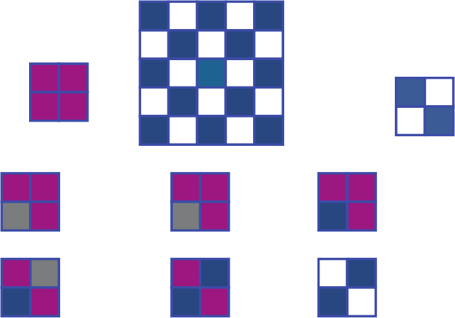
Consider the example in Figure 6.3. The goal is to generate a binary model for a 2 × 2

grid that displays a checkerboard pattern similar to the training image shown at the top of

Figure 6.3. The sequential simulation of this 2 × 2 grid proceeds as follows:

Step 1. Pick any of the four cells.

Step 2. What is the probability of having a blue color in this cell? Since there are not yet

any previously determined cells, that probability is equal to the overall estimated

percentage of blue pixels, in this case 13/25 = 52% because there are thirteen

blue cells and twelve white cells in the training image.

Step 3. Given the 52% probability, determine whether by random drawing a blue or white

color will be given this cell. Suppose the outcome of this random drawing is blue.

P1: OTA/XYZ P2: ABC

JWST061-06 JWST061-Caers March 30, 2011 19:10 Printer Name: Yet to Come

98 CH 6 MODELING SPATIAL UNCERTAINTY

Step 4. Pick randomly another cell.

Step 5. What is the probability of having a blue color in this cell given that the previous

visited cell has been simulated as blue? Now, this depends on the particular be-

lieved arrangement of blue and white cells, that is, the spatial continuity model.

Given the pattern depicted in the training image, the only possible outcome is to

have a blue cell, hence the probability equals 100%.

Step 6. The other two cells will be simulated white for the same argument.

By changing the order in which cells are visited or by changing the random drawing

(steps 3 and 5) a different result will be obtained. For this particular case, there can be

only two possible ﬁnal models each with an almost equal chance of being generated. In

geostatistical jargon, each ﬁnal result is termed a “realization”. In this book it is called an

“Earth model.”

6.3.2 Sequential Simulation Based on Training Images

Figure 6.3 shows that sequential simulation forces a pattern in the 2 × 2 model that is

similar to the pattern of a training image. In terms of actual 3D Earth modeling this means

that the training image expresses the pattern one desires the Earth model to depict. The

sequential procedure explained step-wise above is essentially similar for complex 3D

models with large 3D training images. At each grid cell in the Earth model, the probabil-

ity of having a certain category, given any previously simulated categories, is calculated.

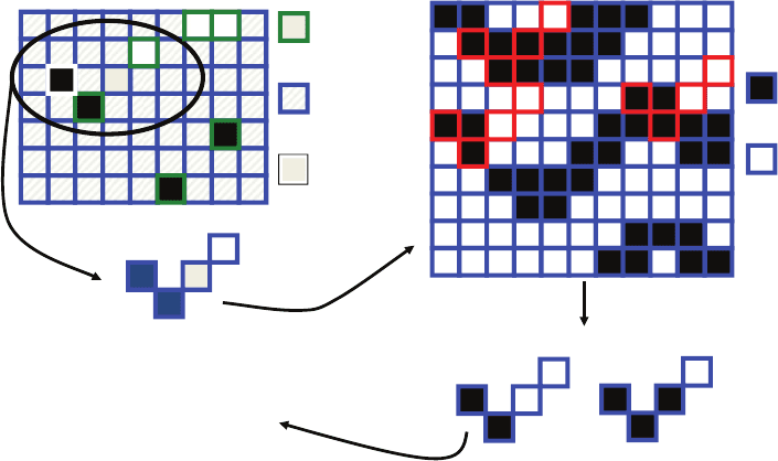
Take for example, the situation in Figure 6.4. The probability of the central cell being

Paern

found

two

mes

“data

event”

Probability for central value to be “Cat 1”=

1/3

Cat 1

Cat 0

Simulaon

grid

Training

image

Previously

simulated

Not

yet

simulated

Cell informed

Point

data

(value

frozen)

Paern

found

one

me

Figure 6.4 Scanning a training image to obtain a conditional probability.

P1: OTA/XYZ P2: ABC

JWST061-06 JWST061-Caers March 30, 2011 19:10 Printer Name: Yet to Come

6.3 TRAINING IMAGE METHODS 99

channel sand given its speciﬁc set of neighboring sand and no-sand data values, is calcu-

lated by scanning the training image in Figure 6.4 for “replicates” of this data event: three

such events are found of which one yields a central sand value, hence the probability of

having sand is 1/3. By random drawing, a category is assigned. This operation is repeated

until the grid is full. This procedure results in a simulated Earth model which will display

a pattern of spatial continuity similar to that depicted in the training image.

In actual cases, data provide local constraints on the presence of certain val-

ues/categories. In sequential simulation, such constraints are handled easily by assigning

(freezing) category values to those grid cells that have point data (= data that inform

directly the cell value) (Figure 6.4). The cells containing such constraints are never vis-

ited and their values never re-considered. The sequential nature of the algorithm forces

all neighboring simulated cell values to be consistent with the data. Unlike object-based

algorithms, sequential simulation methods allow constraining to well data in a single pass

over all grid cells, no iteration is required.

6.3.3 Example of a 3D Earth Model

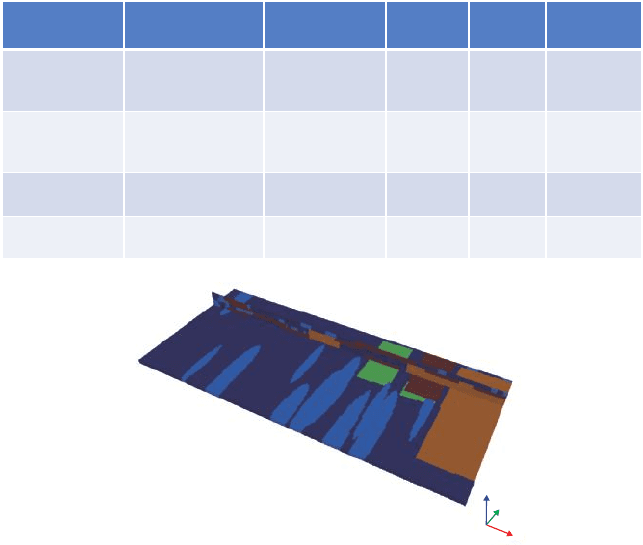
Consider the example of modeling rock types in a tidal dominated system further illus-

trates the concept of importing realistic geological patterns from training images. A grid

of 149*119*15 cells with grid cell size of 40 m*40 m*1 m is considered (Figure 6.5). The

Background

shales

Estuarine

sands

Tida

sand

ﬂats

Transgressive

lags

Tida

bars

Facies

type

Conceptual

descripon

Stragraphy

Length

(m)

Width

(m)

Thickness

()

Tidal

bars

Elo

gate

ellipses

upper

sigmoidal

cros

secon

2000-4000Anywhere 3-7500

Tidal

ﬂats

Sheets

(rectangular)

Anywhere

Ero

sand

bars

610002000

Estuarine

sands

Sheets

(rectangular)

the

reservoir

820004000

Transgressive

lags

Sheets

(rectangular)

the

est

ari

sands

410003000

Figure 6.5 Table with rock type relations and geometrical description. The corresponding train-

ing image was generated using an unconstrained Boolean simulation method.

P1: OTA/XYZ P2: ABC

JWST061-06 JWST061-Caers March 30, 2011 19:10 Printer Name: Yet to Come

100 CH 6 MODELING SPATIAL UNCERTAINTY

model includes ﬁve rock types: shale (50%), tidal sand bars (36%), tidal sand ﬂats (1%),

estuarine sands (10%) and transgressive lags (3%). Using an unconditional object-based

method a training image was constructed using the following geological rules:

Tidal sand ﬂats should be eroded by sand bars.

Transgressive sands should always appear on top of estuarine sands.

An object parameterization for each facies type, except the background shale, is given

in Figure 6.5.

In addition to these geological rules and patterns, trend information is available from

well-logging and seismic data. Trend information is usually not incorporated in the train-

ing image itself but input as additional constraints for generating an Earth model. Since

in sequential simulation an Earth model is built cell-by-cell, the trend information can

be enforced into the resulting Earth model directly, no iteration is required. The training

image needs only reﬂect the fundamental rules of deposition and erosion (the geological

concept) and needs not be constrained to any speciﬁc data (well, vertical and aerial pro-

portion variations, and seismic data). In geostatistical jargon, the training image contains

the nonlocations speciﬁc stationary information (patterns, rules), while reservoir speciﬁc

data enforces the trend. In this example, the following trend information was considered:

Because of coastal inﬂuence, sand bars and ﬂats are expected to prevail in the south-east

part of the domain.

Shale is dominant at the bottom of the model, followed by sand bars and ﬂats, whereas

estuarine sands and transgressive lags prevail in the top part.

Using the point data obtained from 140 wells, an aerial proportion map and a vertical

proportion curve are estimated for each category. Figure 6.6 shows a single Earth model

generated using this approach. The model matches the imposed erosion rules, depicted

by the training image of Figure 6.6, matches exactly all data from 140 wells and follows

the trends described by the proportion map and curves. The generated geometries are not

as crisp as the Boolean training image model; there are some limitations as to what this

technique can achieved but the overall joint capability of matching the data and producing

realistic looking 3D models makes this an appealing technique.

6.4 Variogram-Based Methods

6.4.1 Introduction

While generating Earth models using Boolean and training image-based techniques is

relatively easily to explain and understand, generating an Earth model with a variogram

is less straight forward and requires a lot theory that will not be covered here. The aim,