Caers J. Modeling Uncertainty in the Earth Sciences
Подождите немного. Документ загружается.

P1: OTA/XYZ P2: ABC
JWST061-06 JWST061-Caers March 30, 2011 19:10 Printer Name: Yet to Come
6.4 VARIOGRAM-BASED METHODS 101
Pla
n
view
of
gri
d
with
locaon
of
th
e
140
wells
1
0
Backgroun
d
shale
San
d
bars
Estuarin
e
sands
Fa
c
ie
s
model
Ver
c
a
l
proporon
curves
Backgroun
d
shale
San
d
bars
Estuarin
e
sands
Aeria
l
proporon
maps
N
N
z
y
x
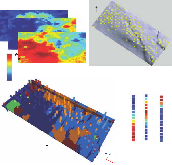
Figure 6.6 Aerial proportion map and vertical proportion curves, a single simulated facies model
constrained to data from 140 wells and reflecting the structure of the training image shown in
Figure 6.5.
however, is similar: to create an Earth model such that when the variogram of the cell val-
ues generated is calculated, we get back approximately the variogram that was obtained
from data or other information. Evidently, there are many such models that can be cre-
ated. To get at least some insight in how this is done it is necessary to discuss the theory
of linear (spatial) estimation first.
6.4.2 Linear Estimation
In linear estimation the goal is to estimate some unknown quantity as a linear combination
of any data available on that quantity. We use weights
␣
z
∗
(u) =
n
␣=1
␣
z(u
␣
)
u and u
␣
denote locations in space. If this is applied to spatial problems then it is
termed spatial estimation. The goal of estimation is to produce a single best guess of this
P1: OTA/XYZ P2: ABC
JWST061-06 JWST061-Caers March 30, 2011 19:10 Printer Name: Yet to Come
102 CH 6 MODELING SPATIAL UNCERTAINTY
unknown. The estimate z* produced will depend on what is considered “best,” but we
will not further discuss this notion as (1) it is for more advanced statistics books and (2)
it is not necessarily important for modeling uncertainty, whose goal is not to get a single
best guess but to study alternatives. Firstly, some “old” methods for performing linear
estimation are discussed, which are actually suboptimal compared to a technique which
is termed “kriging.”
6.4.3 Inverse Square Distance
Considering that spatial estimation is being performed, it makes sense to include the
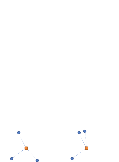
distance between the unknown and the sample data in this process. Consider a simple
example of estimating an unknown from three sample points (Figure 6.7, case 1). In Case
2, the distances are still the same but the data configuration has changed.
It makes intuitive sense that the larger the distance taken the smaller the weight that
will be obtained. A proposal for
␣
is:
i
=
1
h
2
i0
3
j=1
1
h
2
j0
e.g.
3
=
1
h
2
30
1
h
10
2
+
1
h
20
2
+
1
h
30
2
Or, for inverse distance:
i
=
1
h
i0
3
j=1
1
h
j0
The Euclidean distance h does not reveal much about the geology itself, it is just a
distance, recall Figure 5.7. A simple improvement would be, therefore, to account for
geological distance as follows:
i
=
1
␥
(
h
i0
)
3
j=1
1
␥
h
j0
z(u
1
)
z(u
2
)
z(u
3
)
z(u) ?
h
10
h
30
h
20
Cas
e
1
z
(
u
1
)
z(u
2
)
z
(u
3
)
z(u) ?
h
10
h
30
h
20
Case 2
Figure 6.7 Two estimation cases with different data configurations.
P1: OTA/XYZ P2: ABC
JWST061-06 JWST061-Caers March 30, 2011 19:10 Printer Name: Yet to Come
6.4 VARIOGRAM-BASED METHODS 103
However, even with this modified distance, the inverse distance is not the best tech-
nique. Consider a modified situation in Figure 6.7 (case 2). If either situation (data con-
figuration) could be chosen for estimating the unknown, which one would be preferred?
While intuitively case 1 appears more favorable, since samples are more evenly spread
out, inverse distance methods give the same weight to samples 1 and 2 in both cases. This
is a problem, since it is known that the information shared by sample 1 and 2 in case 2
are redundant towards estimating the unknown. Indeed, if two samples are close together,
then it would be expected that they are highly correlated. Hence, one sample might be
enough to contribute information towards estimating the unknown. Inverse distance meth-
ods do not take into account the redundancy of information. In the next section, Kriging
is introduced as a technique that accounts for this redundancy when assigning weights.
6.4.4 Ordinary Kriging
Ordinary Kriging is a spatial interpolation technique that fixes many of the problems of
inverse distance estimation. There is nothing “ordinary” about Ordinary Kriging. It is
just a name to distinguish it from the many other forms of Kriging. In this section, the
technical mathematical details of Kriging will not be discussed. Rather, an attempt is
made to outline the properties of Kriging and learn exactly what it does. These properties
can be summarized in one statement:
Kriging is the “best” linear, unbiased estimator accounting for the correlation between the
data and the unknown and the redundancy of information carried by the data.
“best” can mean a lot of things. In fact, it is necessary to decide what “best” is. In Kriging,
the goal is to estimate the unknowns at all locations that have not been sampled. Ideally,
the estimates should be as close as possible to the true unknown values.
Kriging is a linear estimator, such that the average squared error between the true value
and the estimate is as small as possible. For example, if the inverse distance method was
applied, then it would be found that the average squared error is larger. The average here
is taken over all unsampled locations.
Moreover, Kriging provides an unbiased estimate. That is, if Kriging is repeated a large
number of times, then on average, the errors that are made will be close to zero. It makes
sense that Kriging makes use of the correlation between the data and the unknown value
that one want to estimate. Kriging, however, also accounts for the correlations in the data.
To find the weights,
␣
, which are needed to calculate the estimate, Kriging meth-
ods essentially solve a linear system of equations. For a simple problem with three data
values, as in Figure 6.7, the system looks as follows:
⎡
⎣
Var ( Z ) C(h
12
) C(h
13
)
C(h
12
)Var(Z) C(h
23
)
C(h
13
) C(h
23
)Var(Z)
⎤
⎦
⎡
⎣
1
2
3
⎤
⎦
=
⎡
⎣
C(h
01
)
C(h
02
)
C(h
03
)
⎤
⎦
This Kriging matrix is also termed the redundancy matrix, since it measures the redun-
dancy between data points. Recall that C() is the covariance function, defined in chapter 5.

P1: OTA/XYZ P2: ABC
JWST061-06 JWST061-Caers March 30, 2011 19:10 Printer Name: Yet to Come
104 CH 6 MODELING SPATIAL UNCERTAINTY
6.4.5 The Kriging Variance
Every estimation method makes errors. A best guess is never equal to the true value,
unless the true value is sampled. This error has to be lived with, but at least we would
like to have an idea of how much error on average is being made. The Kriging variance
provides an idea of the magnitude of the error. In essence, if the estimation study was
repeated many times, then the Kriging variance would estimate the variance of the differ-
ence between true and estimated values. Without much ado we simply list the equation
emanating from theory for the ordinary Kriging variance:
2
OK
= Var
(
Z
)
−
n
␣=1
␣
C
(
h
0␣
)
6.4.6 Sequential Gaussian Simulation
6.4.6.1 Kriging to Create a Model of Uncertainty
The goal of Kriging is to provide a single best guess for the value at an unsampled lo-
cation. This is at all not the goal in this book, which is to model uncertainty. Uncer-
tainty requires providing multiple alternatives to the true unknown value or to provide a
probability distribution that reflects the lack of knowledge of that truth. This probability
distribution needs to be conditioned to the available data. Recall that in the 3D training
image approach this conditional probability distribution was lifted directly from the 3D
training image. Hence, this probability depends on the spatial variation seen in the 3D
training image. In variogram-based Earth modeling Kriging can be used to derive such
probability distribution as follows.
Firstly, it is necessary to assume that a variogram or covariance model of the spatial
variable being studied is provided. Assume (and this is a considerable assumption) that
the conditional distribution about any unsampled location is a Gaussian/normal distribu-
tion function. Then, if it is known what the mean is of that Gaussian distribution and the
variance, then we have a model of uncertainty for the unsampled value in terms of that
(Gaussian) conditional distribution. A good candidate for determining this mean is the
Kriging estimate, since as a best guess it provides what can be expected “on average”
at this location. The Kriging variance is a good candidate for informing the variation
around this “on average” value. Note that the Kriging weights depend on the variogram
(or covariance), so the model of spatial continuity has been included in our uncertainty
analysis. Once it is known how to determine this conditional Gaussian distribution, it is
possible to proceed with sequential simulation as outlined above. This technique is then
termed “sequential Gaussian simulation.”
6.4.6.2 Using Kriging to Perform (Sequential) Gaussian Simulation
In order to perform sequential Gaussian simulation it is necessary to assume that all distri-
butions are standard Gaussian. This also means that the marginal distribution, or in other
P1: OTA/XYZ P2: ABC
JWST061-06 JWST061-Caers March 30, 2011 19:10 Printer Name: Yet to Come
6.4 VARIOGRAM-BASED METHODS 105
words, the histogram of the variable is (standard) Gaussian. This is rarely the case; most
samples obtained from the field are not Gaussian. To overcome this issue, a transforma-
tion of the variable into a Gaussian variable is performed prior to stochastic simulation.
In Chapter 2 such a technique for data transformation was discussed. Then, when the
simulation is finished, a back transformation is performed, which does the exact opposite
of the first transformation. The complete sequential Gaussian simulation algorithm can
now be summarized as follows:
1 Transform any sample (hard) data to a standard Gaussian distribution.
2 Assign the data to the grid.
3 Define a random path that loops over all the grid cells.
4 For each grid cell:
a Determine by Kriging the weights assigned to each neighboring data value or previ-
ously simulated value.
0.14
0.12
0.1
0.08
0.06
0.04
0.02
02040
60 80
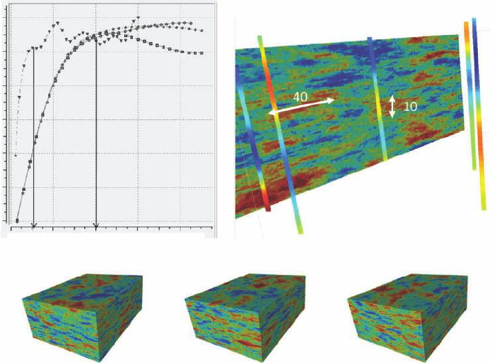
Figure 6.8 Three 3D Earth models generated using sequential Gaussian simulation (bottom).
The variogram calculated from one model for two horizontal and the vertical directions (top).
P1: OTA/XYZ P2: ABC
JWST061-06 JWST061-Caers March 30, 2011 19:10 Printer Name: Yet to Come
106 CH 6 MODELING SPATIAL UNCERTAINTY
b Determine the Gaussian distribution with as mean the Kriging mean and as variance
the Kriging variance.
c Draw a value of that distribution.
5 Back transform all the values into the original distribution.
Figure 6.8 shows an example of sequential simulation. The input variogram used is
isotropic in the horizontal direction with a range of 40 grid cells, the vertical direction
has a range of 10 grid cells; there is no nugget effect. Samples of the variable (poros-
ity in this case) are available along wells. The three resulting Earth models reflect this
variogram as well as being constrained to the sample data values.
Further Reading
Chiles, J.P. and Delfiner, P. (1999) Geostatistics: Modeling Spatial Uncertainty, John Wiley & Sons,
Inc.
Daly, C. and Caers, J. (2010) Multiple-point geostatistics: an introductory overview. First Break, 28,
39–47.
Hu, L.Y. and Chugunova, T. (2008) Multiple-point geostatistics for modeling subsurface heterogeneity:
A comprehensive review. Water Resources Research, 44, W11413. doi:10.1029/2008WR006993.
Lantuejoul, C. (2002) Geostatistical Simulation, Springer Verlag.
P1: OTA/XYZ P2: ABC
JWST061-07 JWST061-Caers April 6, 2011 13:20 Printer Name: Yet to Come
7
Constraining Spatial Models of
Uncertainty with Data
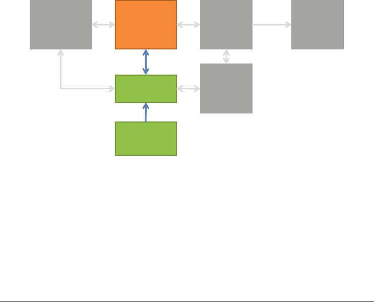
A common problem in building Earth models and constraining models of uncertainty lies in
combining data sources that are indirect and at a different scale from the modeling scale with
data that provide more direct information, such as those obtained through sampling.
Physical
model
Spaal
Stochasc
model
Spaal
Input
parameters
Forecast
and
decision
model
Physical
input
parameters
Raw
observaons
Data sets
response
uncertain
uncertain
uncertain certain or uncertain
uncertain/error
uncertain
uncertain
7.1 Data Integration
Data integration refers to the notion that many different sources of information are avail-
able for modeling a property or variable of interest. The question then is on how to com-
bine these sources of information to model the spatial variable of interest. Ideally, the
more data we have, the smaller the uncertainty on the variable of interest. The latter de-
pends on how much information each data source carries about the unknown and how
Modeling Uncertainty in the Earth Sciences, First Edition. Jef Caers.
© 2011 John Wiley & Sons, Ltd. Published 2011 by John Wiley & Sons, Ltd.
107
P1: OTA/XYZ P2: ABC
JWST061-07 JWST061-Caers April 6, 2011 13:20 Printer Name: Yet to Come
108 CH 7 CONSTRAINING SPATIAL MODELS OF UNCERTAINTY WITH DATA
redundant this source of information is with respect to other data sources in determining
this unknown. In this book, two types of information have so far been dealt with: (1)
hard data or direct measurements of the variable of interest at the scale at which mod-
eling takes place and (2) spatial continuity information, that is, information on the style
of spatial distribution of the property of interest as modeled in a variogram, Boolean
model or 3D training image model. In this chapter all other information sources are con-
sidered. Common examples in Earth modeling are remote sensing data or geophysical
measurements. A common problem in building Earth models and constraining models of
uncertainty lies in combining data sources that are indirect and at a different scale than
the modeling scale with data that provide more direct information, such as those obtained
through sampling. Two approaches are discussed: (1) a probabilistic approach, which is
relatively straightforward and easy to apply but may neglect certain aspects of the rela-
tionship between what is modeled and the data, and (2) an inverse modeling approach,
which can include more information but may often be too CPU demanding or basically
“overkill” for the decision problem we are trying to solve. In this chapter, we consider that
“raw measurements” have been converted into “datasets” suitable for modeling. It should
be understood that such a conversion process may be subject to a great deal of processing
and interpretation, hence the data sets themselves are uncertain. To represent this uncer-
tainty, multiple alternative data sets could be generated. In the rest of the chapter, methods
to deal with one of these alternative data sets are discussed.
7.2 Probability-Based Approaches
7.2.1 Introduction
Assume that we have various types of data about the 3D Earth phenomena we are trying to
model, such data can often be classified in two groups: samples and geophysical surveys.
By samples we mean a detailed analysis at a small scale (although scale is here relative to
the modeling problem); these could be soil samples, core samples, plugs, well-logging,
point measurements of pressure, air pollutions and so on. By geophysical measurements
we understand the various remote sensing techniques applied to the Earth to gather an
“image” of the Earth or surface being modeling (e.g., synthetic aperture radar, seismic,
ground penetrating radar). There may be various geophysical data sources (electromag-
netic, seismic, gravity) and various point sources. Other type of measurements may be
available that are indicators of what is being modeled: in general such information is
named “soft information.” In this section, the following are addressed:
r
How to use data sources such as geophysical measurements or “soft information” in
general to reduce uncertainty about what is being modeled (and hopefully about deci-
sions being made, see also Chapter 11).
r
How to account for the “partial information” that such data sources provide.
r
How to combine several data sources (e.g., several geophysical sources, or point sam-
ples with geophysical sources) each one of which provides only partial information.
P1: OTA/XYZ P2: ABC
JWST061-07 JWST061-Caers April 6, 2011 13:20 Printer Name: Yet to Come
7.2 PROBABILITY-BASED APPROACHES 109
A data source often provides only partial information about what we are trying to
model. For example, seismic data (Chapter 8) does not provide a measurement of porosity
or permeability, properties important to flow in porous media; instead, it provides mea-
surements that are indicators of the level of porosity. Satellite data in climate modeling
do not provide direct, exact information on temperature, only indicators of temperature
changes. Given these criteria, we will proceed in two steps in order to include these data
in our model of uncertainty:
1 Calibration step: how much information is contained in each data source? Or, what is
the “information content” of each data source?
2 Integration step: how do we combine these various sources of information content
into a single model of uncertainty?
7.2.2 Calibration of Information Content
The amount of information contained in a data source is dependent on many factors, such
as: the measurement configuration, the measurement error, the physics of the measure-
ment, the scale of modeling, and so on.
The first question that should be asked is: how do we model quantitatively the infor-
mation content of a data source. In probabilistic methods a conditional distribution is
used (Chapter 2). Recall that a conditional distribution P(A|B) models the uncertainty of
some target variable A, given some information B. In our case B will be the data source
and A will be what is being modeled. Recall also that if P(A|B) = P(A) then B carries no
information on A. The question now is how is P(A|B) determined?
To determine such conditional probability, more information is needed, more specif-
ically, we need data pairs (a
i
, b
i
), that is, mutual or joint observations of what we are
trying to model and the data source. This means that at some limited set of locations it is
necessary to have observed the true Earth as well as the data source. In many applications,
at the sample locations, it is possible to have information on A as well as B.
For example, from wells, there may be measurements of porosity and from seismic
measurements of seismic impedance (or any other seismic attribute) in 3D (such as shown
in Figure 7.1). This provides pairs of porosity and impedance measurements that can be
used to plot a scatter plot, such as shown in Figure 7.2. In this scatter plot P(A|B) can now
be calculated, where the event “A = (porosity < t)”, for some threshold t, and “B = (s <
impedance < s + s)”, as shown in Figure 7.2. In this way a new function is created:
P(A|B) = (t, s)
Once we have this function, the conditional probability for any t and any s can be
evaluated. This function is a “calibration function” that measures how much information
impedance carries about porosity. There are many other ways to get this function. Physical
approaches such as rock physics may provide this function, or one may opt for statistical
techniques (e.g., regression methods such neural networks) to “lift” this function from a
data set belonging to another field if what occurs in that field is deemed similar.
P1: OTA/XYZ P2: ABC
JWST061-07 JWST061-Caers April 6, 2011 13:20 Printer Name: Yet to Come
110 CH 7 CONSTRAINING SPATIAL MODELS OF UNCERTAINTY WITH DATA
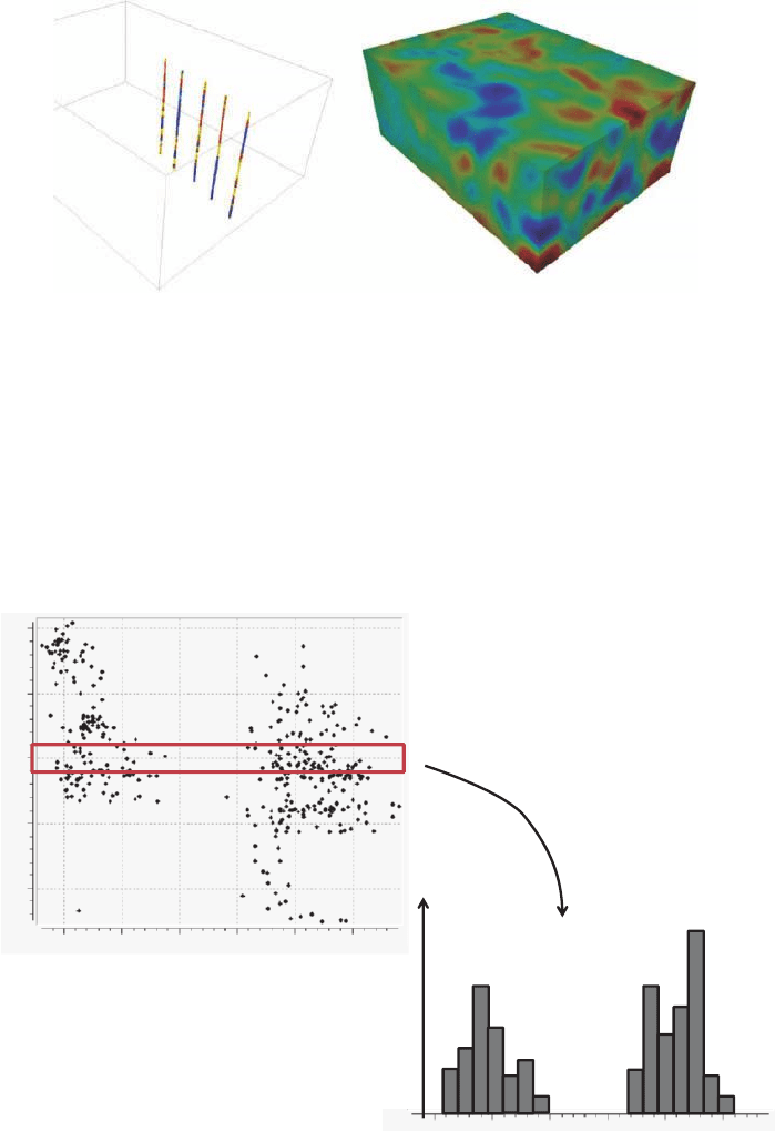
Figure 7.1 Calibration data set: samples providing detailed but only local information (left);
a geophysical image of the earth providing a fuzzy but global insight (right). At the sample
locations we have both sets of observations.
7.2.3 Integrating Information Content
Consider now the situation where several such calibrations have been obtained because
many data sources are available. In other words, several P(A| B
1
), P(A| B
2
), .... have been
obtained. The next question is: how do we combine information from individual sources
freq
Lo
g
impedance
porosity
porosity
His
t
ogra
m
of
porosity
dat
a
in
this
window
7.5
7
6.5
6
5.5
0.05 0.1 0.15 0.2 0.25 0.3
0.05 0.1 0.15 0.2 0.25 0.3
Figure 7.2 Calibration of porosity from seismic using a scatter plot. By considering porosity
within a given window of seismic impedance, it is possible to calculate the frequencies of porosity
that are less than a certain threshold value from the histogram shown.