Carranza E. Geochemical anomaly and mineral prospectivity mapping in GIS
Подождите немного. Документ загружается.

Spatial Data Models, Management and Operations 37
size is equivalent to area.
Distance calculation is important in many GIS analyses for mineral exploration. For
example, Seoane and De Barros Silva (1999) introduced a drainage sinuosity index to
rank gold-anomalous catchment basins. They calculated sinuosity index as ratio of total
length of drainages in a segment basin to distance between a sampling point represented
by a segment basin and the most upstream point of that segment basin. Distance
calculations are also important in quantifying spatial associations between mineral
deposits and certain geological features (see Chapter 6).
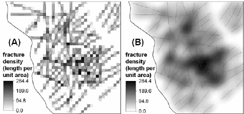
Another form of measurement is point or line density, which is the number of points
or the total length of lines, respectively, per unit area. Fig. 2-11A shows a map of
fractures and the corresponding fracture density created by a simple method of
measuring total length of fractures per unit area. Note the blocky character of the simple
fracture density map, from which it is evident which pixels contain a facture segment. A
smoother facture density map (Fig. 2-11B) could be achieved via a gridding method (see
further below). It is clear in the example that a fracture density map, for example, is a
form of transformation of line or point geo-objects into area or surface geo-objects. Point
density calculation is an important concern in the analysis of spatial association between
mineral deposits and certain geological features (Chapter 6). In such analysis, linear
geological objects are represented as or transformed into polygonal features.
Transformations
Most GIS operations on spatial data can be considered transformations. In fact,
calculation of density of point or linear geological features is transformation of the 0-D
or 1-D, respectively, of these geo-objects into 2-D. Perhaps the most important type of
transformation in a GIS is conversion of geographical coordinates, in which most spatial
data are probably originally stored, into planar coordinates of suitable map projections
(Maling, 1992). Geometric corrections of satellite imagery and transformations of
various raster maps into a common pixel size are also important in GIS studies. Such
transformations, known as resampling (Mather, 1987), ensure that map layers in a GIS
are properly georeferenced. Transformations to derive digitally-encoded data, such as
Fig. 2-11. Fractures (linear features) and fracture density estimated as total length per unit area or
pixel (A) and then smoothed via a gridding method (B).
38 Chapter 2
line generalisations, are important in capturing spatial data (McMaster and Shea, 1992;
Garcia and Fdez-Valdivia, 1994). There are many other types of transformations in a
GIS. Bonham-Carter (1994) provides elaborate discussions on the concepts and
algorithms of many different types of spatial data transformations that are applicable to
geoscience modeling in general.
The discussion here concentrates on spatial data transformations that are more
directly and usually involved in mapping of geochemical anomalies and mineral
prospectivity. These are point-to-area, point-to-surface, line-to-area, line-to-surface,
area-to-point, area-to-area and surface-to-area transformations. The last two
transformations are handled via re-classification operations (see above). Some of these
transformations may require conversion from a vector data model to a raster data model
and vice versa. Detailed discussions on vector-to-raster and raster-to-vector conversions
can be found in Clarke (1995), Mineter (1998) and Sloan (1998). Area-to-point
transformation, for example, can be handled by vector-to-raster conversion, whereby
polygonal geo-objects are converted to pixels and each pixel can treated as a point.
Most geoscience spatial data used in mapping of geochemical anomalies and mineral
prospectivity are recorded as attributes of sampling points (Fig. 2-12A). Because the
objective of most mineral exploration activities is to define anomalous zones rather than
points (except in defining locations for drilling), point-to-area and/or point-to-surface
transformations are required to analyse and model spatial information from point data.
The types of transformations performed depend on the type of geo-objects represented
by point data and on the nature of attribute data. On the one hand, point-to-area
transformations of point data representing geo-objects such as intersections of curvi-
linear structures or locations of mineral deposits can be modeled appropriately by, for
example, point density calculations. On the other hand, point-to-area and point-to-
surface transformations of point data representing qualitative or quantitative attributes
can be modeled by, respectively, non-interpolative transformations or spatial
interpolations. The objective of such transformations is to reconstruct the continuous
field, respectively, which was measured at the sampling points.
Non-interpolative transformations are suitable for point data measured on a nominal
scale. In some cases, such transformations are also applicable to point data measured on
ordinal, interval or ratio scale. Non-interpolative transformations involve creation of
zones of influence around points with assumption of homogeneity of attribute data in
each zone. Bonham-Carter (1994) describes a number of methods of non-interpolative
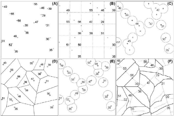
point-to-area transformations, which are briefly reviewed here. The simplest method is
to associate attributes of each point to a rectangular cell in a regular grid. Cells with
more than one point are assigned attributes that are aggregated according to some rule
and depending on measurement scale, whilst cells without points are assigned null
attributes (Fig. 2-12B). This method has been used for regional geochemical mapping
(e.g., Garrett et al., 1990; Fordyce et al., 1993). A modification of representing point data
as rectangular cells is to draw equal-area circular cells centred on points and to assign
attributes of each point to the corresponding circle; zones outside the circles are assigned
null attributes (Fig 2-12C). An advantage of this method is that the size of the circle can
Spatial Data Models, Management and Operations 39
be chosen with subjectivity to represent zone of influence of a point. A disadvantage of
this method is that some circles will overlap, which provides difficulty in deciding
assignment of attributes to overlapping zones. This problem can be overcome by
creating Thiessen or Voronoi or Dirichlet polygons around each point (Fig 2-12D)
(Burrough and McDonnell, 1998). The points can then be represented by Thiessen
polygons restricted to circular zones (Fig 2-12E). Bartier and Keller (1991) represented
stream sediment point data as Thiessen polygons to integrate such data with bedrock
geological data in a GIS analysis. They recognise, however, that representation of stream
sediment data as Thiessen polygons is less appealing intuitively than representation of
such data as sample catchment basin polygons, which is another method of point-to-area
transformation (Fig 2-12F).
Spatial interpolation is involved in point-to-surface transformations of point data
representing continuous variables. Surface models produced by any interpolation method
can be symbolised and visualised by contouring, a subject that is treated thoroughly by
Watson (1992). For a given set of irregularly- or regularly-spaced point data, there are
Fig. 2-12. Point-to-area transformations (adapted from Bonham-Carter, 1994, pp. 146). (A)
Distribution of point data on a map. (B) Points transformed to regular cells. Cells with more than
one point are assigned aggregated (e.g., mean) attributes whilst cells without points are null
attributes. (C) Points transformed to circular cells. Zones defined by overlapping circles are
assigned aggregated attributes. (D) Points transformed to Thiessen polygons. (E) Points
transformed to areas defined by overlap of Thiessen polygons and circular cells. (F) Stream
sediment sample points transformed to sample catchment basins. Dotted lines are streams. Solid
lines are outlines of drainage catchment basins.
40 Chapter 2
several spatial interpolation methods, which can generally be classified as either
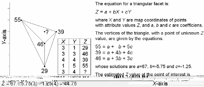
triangulation (i.e., TIN generation) or gridding methods. In triangulation methods, given
control points form vertices of triangles and values at any point are estimated according
to the equation for a triangular facet containing such points (Fig. 2-13). Triangulation
methods are suitable for modeling of topographic, stratigraphic or structural surfaces. In
gridding methods, values of the surface to be modeled are estimated at locations, called
‘grid nodes’, arranged in a regular pattern completely covering area of interest. Grid
nodes are usually arranged in a square pattern and a zone enclosed by four nearest
neighbouring grid nodes is called a ‘grid cell’. The choice of a grid cell size, which
determines accuracy and computing time of a surface model, is largely a subjective
judgment but depends primarily on density and distribution of a given point data set.
Generally, values of the surface at grid nodes are unknown and are estimated using
control points where values of the surface are known. Various gridding methods exist
and their detailed descriptions can be found in several textbooks (e.g., Burrough and
McDonnell, 1998). For each gridding method, the estimation process involves three
essential steps. Control points are first sorted according to their geographic coordinates.
From the sorted controls points, a search is made for control points within a
neighbourhood surrounding a grid node to be estimated. The value of a grid node is
finally estimated by some mathematical function of values of control points within a
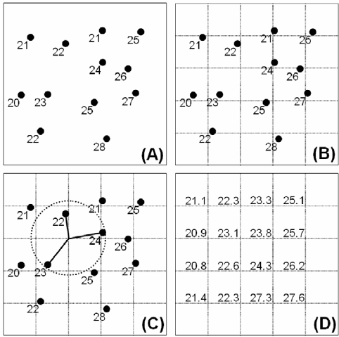
search neighbourhood (which is usually circular or elliptical). An example of a
mathematical function is moving average, whereby for each grid node the average of
values at control points within a search neighbourhood that is ‘moved’ from one grid
node to another is estimated (Fig. 2-14). Values at control points are projected
horizontally to a grid node, where they are weighted and averaged. Weights are
calculated because control points closer to a grid node to be estimated should have more
influence on the estimated value than control points farther away. Of the different
Fig. 2-13. Transformation of data points (at vertices of triangles) into a surface via Delaunay
triangulation. With assumption that an unknown point lies on the plane of a triangular facet, the
value at that point can be estimated based on the equations of the triangle’s vertices.
Spatial Data Models, Management and Operations 41
‘weighted moving average’ methods, inverse distance method and kriging have been
usually applied to model geochemical surfaces. Point-to-surface transformations of
geochemical data by spatial interpolation are applicable in fractal analysis of
geochemical anomalies (see Chapter 4).
Methods of point-to-surface transformations are also applicable to line-to-surface
transformations of linear geo-objects representing continuous variables (e.g., isolines of
elevation). That means all points or samples of points along linear geo-objects are used
in triangulation or gridding methods. In contrast, methods of point-to-area
transformations are not readily applicable to line-to-area transformations, particularly if
linear geo-objects represent qualitative variables. For linear geo-objects representing
qualitative variables (e.g., curvi-linear structures, lithologic contacts, etc.), the idea of
line-to-area transformation is to generate zones of proximity to linear features through an
operation known as buffering or dilation, which depends on distance calculations. Points
or polygons can also be buffered (i.e., point-to-area or area-to-area transformations) if
Fig. 2-14. Transformation of data points into a surface grid. (A) Control data points; each point is
characterised by its x-coordinate (east-west or across page width), y-coordinate (north-south or
down page length), and z-coordinate (value beside a point). Point data are identified by numbering
them sequentially, as read by software, from 1 to i. Thus, a control point i has coordinates x
i
and y
i
and a value z
i
. (B) A regular grid of nodes is superimposed on the map. These grid nodes are also
numbered sequentially from 1 to k. Each grid node has coordinates x
k
and y
k
, and a value to be
estimated z
k
. (C) The value z
k
at a grid node k is estimated from n control points found within a
search neighbourhood, of specified area of influence, centred at k. (D) Completed grid with
estimated values of z
k
.
42 Chapter 2
they represent qualitative variables. Buffering is performed when one intends to
determine spatial associations between locations of mineral deposits and various
geological features (e.g., structures, anomalies). Buffering is among the most common
neighbourhood operations, which are treated briefly below and treated in more detail in
Chapter 6.
Neighbourhood operations
The general objective of a neighbourhood operation is to analyze the characteristics
and/or spatial relationships of locations surrounding some specific (control) locations.
Note that control locations are actually part of the neighbourhood to be analyzed. Thus,
in fact, spatial interpolation techniques are a type of neighbourhood operation, because
they aim to estimate values at unsampled locations based on values at sampled locations.
Most types of neighbourhood operations applied in mapping of geochemical anomalies
and mineral prospectivity are performed using a raster data model, because this ensures
spatial adjacency of control pixels to neighbouring pixels. Buffering, however, may be
performed using either vector or raster data.
Neighbourhood operations applied to raster maps are basically filtering operations.
Filtering can be performed in the time domain, frequency domain or spatial domain.
Filtering in the spatial domain is a basic function in GIS, which is further discussed here.
Filtering operations in the time domain and frequency domain are beyond the scope of
this volume; Davis (2002) provides a clear discussion of filtering operations in the time
and frequency domains as applied to geological data analysis.
Filtering of a raster map involves an equal-sided filter window, also called a “kernel”
or “template”, which moves across a raster map one pixel at a time. A filter has an odd
number of pixels on each of its sides so that it defines a symmetrical neighbourhood
about the central pixel (Fig. 2-15). The simplest filter is a square of 3x3 pixels. Each
pixel visited by a filter becomes the control location in a neighbourhood and a new value
is calculated for that pixel according to certain mathematical ‘search’ functions that are
desired to characterise that neighbourhood.
There are three basic elements in a neighbourhood operation – the control pixel, the
neighbouring pixels and the search function to be applied to the neighbourhood. Because
there are four general types of spatial data – ratio, interval, ordinal, nominal – the choice
of mathematical search functions used in filtering operations depends on the type of data
being studied. Note also that if a function can be applied to any type of data in the order
as listed above, then that function can also be applied to the preceding type of data. The
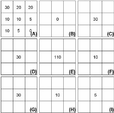
following discussion details examples of eight mathematical search functions, which are
described along with their results for data in Fig. 2-15A.
The data in Fig. 2-15A can be ratio, interval or ordinal. A MINIMUM function
returns to the central pixel the value of the pixel in the neighbourhood with the lowest
value (Fig. 2-14B). The MINIMUM function is often used in a BOOLEAN search query
(true or false) to find ‘false pits’ (single pixel depressions) in a digital elevation model
(DEM) before performing runoff simulations. A MAXIMUM function returns to the
central pixel the value of the pixel in the neighbourhood with the highest value (Fig. 2-
Spatial Data Models, Management and Operations 43
15C). The MAXIMUM function can be used to find, for example, locations with highest
probability of deposit-type occurrence in a mineral prospectivity map. A RANGE
function returns to the central pixel the difference between highest and lowest values in
the neighbourhood (Fig. 2-15D). The RANGE function can be used, for example, to find
the range of metal concentrations surrounding every location in a soil geochemical map,
which may indicate locations with high geochemical contrast. A SUM function returns
to the central pixel the sum of the pixel values in the neighbourhood (Fig. 2-15E). The
SUM function is useful in measuring density of geo-objects in a map. A MEDIAN
function returns to the central pixel the median of pixels values in the neighbourhood
(Fig. 2-15F). The MEDIAN function can be used, for example, to smooth values in a
map; it serves a similar purpose to using an AVERAGE function. The AVERAGE
function usually returns an integer value rather than a real value, and thus it is not
suitable for interval or ordinal data. A MINORITY function returns to the central pixel
the pixel value that occurs least frequently in the neighbourhood (Fig. 2-15G). The
MINORITY function is rarely used. A MAJORITY function returns to the central pixel
the pixel value that occurs most frequently in the neighbourhood (Fig. 2-15H). The
MAJORITY function can be used to replace missing values in a map; for example, to
assign the most common lithologic unit in a neighbourhood. Note that unique interval or
ordinal values can be assigned to lithologic units instead of their names, because the
latter type of data are not amenable to mathematical operations. A DIVERSITY (or
VARIETY) function returns to the central pixel the number of different pixel values in
the neighbourhood (Fig. 2-15I). The DIVERSITY function can be used, for example, to
Fig. 2-15. Neighbourhood operations with mathematical search functions. (A) Example raster map
data. (B) Result of a MINIMUM function. (C) Result of a MAXIMUM function. (D) Result of a
RANGE function. (E) Result of a SUM operation. (F) Result of a MEDIAN function. (G) Result
of a MINORITY function. (H) Result of a MAJORITY function. (I) Result of a DIVERSITY
function.
44 Chapter 2
find edges of polygons of different lithologic units whereby it returns a value of [1] for
interior of a lithologic unit, [2] along the contacts of two lithologic units, and [3] or
higher values where three or more lithologic units join (cf. Mihalasky and Bonham-
Carter, 2001).
The preceding examples belong to the aggregation type of neighbourhood operations.
Clear introductory discussions of other different types of spatial filters, particularly those
used in raster image analysis, and the functions associated with such filters can be found
in Bonham-Carter (1994, p. 204-212). Other types of neighbourhood operations involve
‘spread’ or ‘seek’ computations. Spread computations are applicable, for example, to
flood inundation studies (e.g., Peter and Stuart, 1999) or environmental pollution studies
(e.g., Haklay, 2007). Seek computations are applicable, for example, to hydrological
studies (e.g., Vieux, 2004).
Map overlay operations
The previously discussed operations on spatial data – spatial query and selection,
classification and re-classification, measurements, transformations, neighbourhood – are
usually applied to analyze spatial patterns of interest in single maps of geoscience spatial
data sets. However, the previously discussed operations could also actually involve at
least a pair of maps. For example, selection of stream sediment samples in zones
underlain by certain lithologic units (Fig. 2-8) involves a map of stream sediment sample
locations and a lithologic map. In addition, mapping of stream sediment sample
catchment basins via a neighbourhood operation involves a map of stream sediment
sample locations, a map of drainage lines and a DEM. These examples show that map
overlay operations are implicitly involved in some of the previously discussed operations
on spatial data. Map overlay operations are perhaps the most important of all GIS
functionalities. There are two important conditions that must be fulfilled in order to
perform overlay operations: (1) maps are georeferenced to the same coordinate system;
(2) maps must overlap and thus pertain to the same study area. The principle in overlay
operations is to integrate maps of certain attributes of every location in order to produce
a map of new attributes for every location.
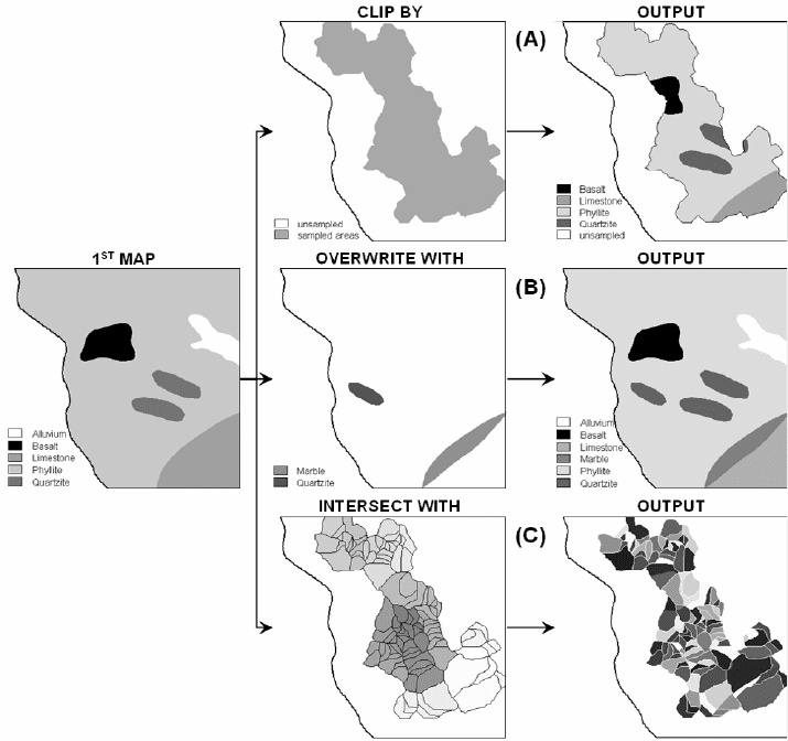
The three most common overlay operations are clip, overwrite and intersect (Fig. 2-
16). The clip operation, which is also called an impose operation, restricts the spatial
extent of the first map to the spatial extent of the second map (the clip map) (Fig. 2-
16A). The clip operation is useful, for example, to retrieve from a source thematic map
spatial data pertaining to a study area. The clip operation does not result in a new
attribute table; the output map adopts the attribute table of the first map. The overwrite
operation, which is also called a stamp operation, adopts the data from the first map
except where there are data in the second map; data in the second map take priority in
the output. The overwrite operation is useful, for example, to update an existing
lithologic map with recent results of lithologic mapping (Fig. 2-16B). The overwrite
operation results in an attribute table for the output map only if the second map has new
data attributes. Creation of a new attribute, however, is not necessary if the attribute
table of the first map is updated initially so that it can be associated with the second map.
Spatial Data Models, Management and Operations 45
The intersect operation, which is also called the cross or spatial join operation, is
perhaps the most standard of all overlay operations. The intersect operation results in a
collection of all possible intersections between geo-objects in the two input maps (Figs.
1-4 and 2-16C). It is useful, for example, in the process of integrating lithologic
information in catchment basin analysis of stream sediment geochemical anomalies
(Chapter 5). The intersect operation is applicable not only to polygonal geo-objects but
also to linear and point geo-objects. If a map of polygonal geo-objects is intersected with
a map of linear geo-objects, then the output map contains only linear geo-objects. The
output geo-objects in an intersect operation adopt the geometry of geo-objects with the
Fig. 2-16. Two-map overlay involving a geological map as common first map and different second
maps. (A) Geological map is clipped by map of an area sampled with stream sediments (see Figs.
2-7A and 2-9A). (B) Geological map is overwritten with a map of recently delineated lithologic
units. (C) Geological map is intersected with (or crossed with) a map of stream sediment sample
catchment basins. Further illustration of the intersect operation is shown in Fig. 2-17.
46 Chapter 2
lowest spatial dimension in one of the input maps. The intersect operation always results
in an attribute table that is associated with the output map.
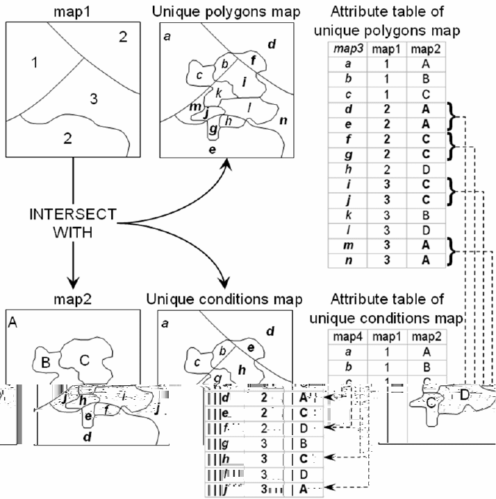
There are two types of intersect operations, one type results in a unique polygons
map and the other type results in a unique conditions map (Fig. 2-17). An intersect
operation that results in a unique polygons map assigns a unique attribute (e.g., geo-
object number or ID) to each polygon, even if there are polygons having the same or
unique combinations of attributes of the input maps. This type of intersect operation is
common in vector-based GIS software packages. An intersect operation that results in a
Fig. 2-17. Illustrations of result of intersect operation into either a unique polygons map or a
unique conditions map. Individual geo-objects in a unique polygons map having the same
combinations of attributes of the input maps are considered geo-objects of the same class in a
unique conditions map. The latter map has fewer classes than the former map.