Carranza E. Geochemical anomaly and mineral prospectivity mapping in GIS
Подождите немного. Документ загружается.

70 Chapter 3
provide additional controls on the spatial distributions of Mn and As. High background
Mn values and high background to outlying As values occur along a northwest-trending
zone in the western part of the area following the same trend of the epithermal Au
deposit occurrences. Note that the gold deposit occurrences are associated with Mn-
stained silicified veins deposited along northwest-trending faults/fractures that cut
dacitic/andesitic volcano-sedimentary rocks. The As outliers in the northwestern part of
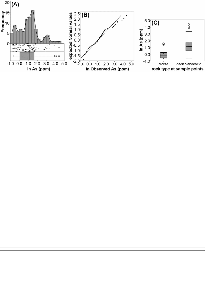
Fig. 3-14. Log
e
-transformed (ln) As data exclusive of censored values, Aroroy district
(Philippines). (A) Histogram and EDA graphics. (B) Normal Q-Q plot showing deviation of the
data from the normal distribution (straight line) model. (C) Boxplots of subsets of the data
according to rock type at sample points.
TABLE 3-II
Classical and EDA statistics log
e
-transformed data subsets according to rock type at sample points,
Aroroy district (Philippines).
Rock type at sample points Element Mean
SDEV Median
MAD
Cu 3.73 0.55 3.72 0.38
Zn 3.45 0.41 3.44 0.30
Ni 2.10 0.61 2.11 0.50
Co 2.50 0.49 2.52 0.32
Mn 6.22 0.37 6.19 0.25
As -0.92 0.78 -1.39 0.00
Aroroy Diorite (at n=38
samples, except the As data*
for n=13 samples)
As* -0.02 0.74 -0.22 0.58
Cu 4.08 0.62 4.08 0.37
Zn 4.08 0.45 4.13 0.24
Ni 2.48 0.55 2.56 0.36
Co 2.85 0.42 2.94 0.28
Mn 6.68 0.41 6.75 0.32
As 0.83 1.41 0.99 0.82
Dacitic/andesitic volcano-
sedimentary rock (at n=97
samples, except the As data*
for n=82 samples)
As* 1.23 1.13 1.16 0.32
*Excluding samples with censored values.
Exploratory Analysis of Geochemical Anomalies 71
the study area are associated with hydrothermally altered volcano-sedimentary rocks.
The maps in Fig. 3-15 also show that low background to censored values of As pertain
mainly to the Aroroy Diorite, so that subdividing the uni-element data sets according to
rock type at sample locations is non-trivial. Moreover, the maps of the As data in Fig. 3-
15 indicate that different forms of the same data set, raw or transformed, influence the
mapping of geochemical anomalies. The following section compares the performance of
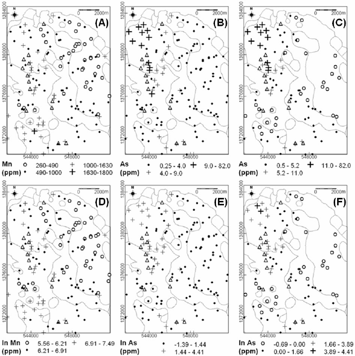
Fig. 3-15. Spatial distributions of selected uni-element data (Aroroy district, Philippines) based on
boxplot-defined classes and EDA mapping symbols. (A) Raw Mn data (boxplot in Fig. 3-10E).
(B) Raw As data with censored values (boxplot in Fig. 3-10F). (C) Raw As data without censored
values (boxplot not shown). (D) Log
e
-transformed Mn data (boxplot in Fig. 3-11E). (E) Log
e
-
transformed As data with censored values (boxplot in Fig. 3-11F). (F) Log
e
-transformed As data
without censored values (boxplot in Fig. 3-14A). Triangles represent locations of epithermal Au
deposit occurrences. Light-grey lines represent lithologic contacts (see Fig. 3-9).

72 Chapter 3
different threshold values (boxplot UW, median+2MAD, mean+2SDEV) in the log
e
-
transformed uni-element data sets, which have more symmetrical distributions than the
respective raw data sets.
Analysis of uni-element threshold values and anomalies
Table 3-III shows the threshold values defined as the mean+2SDEV, median+2MAD
and boxplot UW in each of the raw and log
e
-transformed uni-element data sets. For the
raw uni-element data sets, the threshold values defined by the median+2MAD are always
the lowest, followed by those defined by either the boxplot UW or the mean+2SDEV,
depending on the uni-element data set. For the log
e
-transformed data sets, the threshold
values defined by the median+2MAD are also always the lowest, followed mostly by
those defined by the mean+2SDEV and the threshold values defined by the boxplot UW
are mostly highest, depending on the uni-element data set. These findings about the
ranking of threshold values defined by each of the three methods and per type of data
(raw or log
e
-transformed) are consistent with the findings of Reimann et al. (2005).
Because the log
e
-transformed data approach symmetrical distributions (Fig. 3-12),
the threshold values determined from such data should be used in mapping of anomalies.
The information in Table 3-III already indicates that the median+2MAD threshold values
result in the highest number of anomalies, followed by the mean+2SDEV threshold
values and then by the boxplot UW threshold values. So, for our pathfinder element for
epithermal Au deposits – As – there are no anomalies based on the boxplot UW (Table 3-
III, Fig. 3-11F), whereas anomalies based on the mean+2SDEV and the median+2MAD
have, respectively, poor and good spatial associations with the known epithermal Au
deposit occurrences in the case study area (Fig. 3-16). So, with respect to As anomalies,
which one expects to be present and strong because of the epithermal Au deposits, the
median+2MAD performs best, followed by the mean+2SDEV and then by the boxplot
UW. The same is true even if the censored values in the As data are discarded (Table 3-
TABLE 3-III
Threshold values defined as mean+2SDEV, median+2MAD and boxplot UW of raw and log
e
-
transformed uni-element data set for n=135 samples (except As*, for which n=95), Aroroy district
(Philippines).
Mean+2SDEV Median+2MAD Boxplot UW
Raw Antilog
e
Raw Antilog
e
Raw Antilog
e
Cu 139.72 184.93 96 120.30 136 200
Zn 121.76 139.77 88 108.85 113 187
Ni 26.31 34.81 22 26.58 30 42
Co 32.06 43.73 26 28.50 36 42
Mn 1461.93 1719.86 1120 1380.22 1630 1800
As 25.86 27.66 4 14.73 9.0 82.0
As* 30.89 29.96 7 11.94 11.0 48.9
*Excluding samples with censored values.
Exploratory Analysis of Geochemical Anomalies 73
III). For the other elements under study, the threshold values based on the boxplot UW
mostly indicate absence of anomalies (Fig. 3-11), whereas threshold values based on
either the mean+2SDEV or the median+2MAD mostly indicate presence of anomalies.
However, the threshold defined by the mean+2SDEV of log
e
-transformed Co values is
greater than the maximum value in that data set (Table 3-III), suggesting that threshold
values based on the mean+2SDEV can be misleading. In the study area, there are likely
no anomalies of Ni and Co but there are likely weak anomalies of Cu, Zn and Mn
associated with the epithermal Au deposit occurrences. So, with respect to Ni and Co
anomalies, which one expects to be absent, the boxplot UW performs best, followed by
the mean+2SDEV and then by the median+2MAD. Finally, with respect to Cu, Zn and
Mn anomalies, which one expects to be present but perhaps weak, the mean+2SDEV
apparently performs best, while the median+2MAD and the boxplot UW, respectively,
over-estimate and under-estimate the anomalies.
The results from each of the whole log
e
-transformed uni-element data sets suggest
that each of the three methods performs differently depending on the actual anomalies
that are likely to be present (or absent) in an area. Reimann et al. (2005) pointed out that
the boxplot UW threshold performs adequately in cases where there are ‘actually’ less
than 10% outliers, whereas the median+2MAD performs adequately in cases where there
are ‘actually’ at least 15% outliers. Although the median+2MAD of the whole log
e
-
transformed As data set performed best among the three methods, in Fig. 3-16B there are
only 11 (or 8.1%) anomalous samples out of the total 135 suggesting that such an
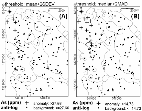
Fig. 3-16. Anomalies in the log
e
-transformed As data set, Aroroy district (Philippines) based on
threshold defined as (A) mean+2SDEV and (B) median+2MAD. There are no As anomalies
according to the boxplot UW (see Fig. 3-11F). Triangles represent locations of epithermal Au
deposit occurrences. Light-grey lines represent lithologic contacts (see Fig. 3-9).

74 Chapter 3
anomaly map is probably not optimal. Therefore, it is instructive to study further
anomalies based on data subsets according to, say, rock type at sample locations.
Table 3-IV shows the threshold values defined as the mean+2SDEV, median+2MAD
and boxplot UW in the individual log
e
-transformed uni-element data subsets according to
rock type at sample locations. As in Table 3-III, the threshold values defined by the
median+2MAD are always the lowest, followed by those defined by either the boxplot
UW or the mean+2SDEV, depending on the element and data subset. The uni-element
threshold values for samples in areas underlain by diorite are probably not physically
meaningful because they are based on only 38 samples. For example, the median+2MAD
threshold for As is equivalent to the minimum (i.e., censored) data value (0.25) in the
data subset for samples in areas underlain by diorite, suggesting that all As values in the
data subset are anomalous. For the samples in areas underlain by dacitic/andesitic rocks,
the threshold values for Cu, Co and Mn based on the mean+2SDEV are greater than the
respective maximum values, suggesting that threshold values based on the mean+2SDEV
can be misleading. The boxplot-defined threshold for As in samples underlain by
dacitic/andesitic rocks is equivalent to the maximum data value (82), suggesting that
there are no As anomalies in the data subset.
The problems with the threshold values for As defined by each of three methods for
the two data subsets according to rock type at sample location are caused by the
censored values. By excluding the censored As values, the threshold values for As
TABLE 3-IV
Threshold values defined as mean+2SDEV, median+2MAD and boxplot UW of the log
e
-
transformed uni-element data subsets according to rock type at sample point, Aroroy district
(Philippines).
Rock type at
sample points
Element
Antilog
e
of
Mean+2SDEV
Antilog
e
of
Median+2MAD
Antilog
e
of
boxplot UW
Cu 125.21 88.23 106
Zn 71.52 56.83 71
Ni 27.66 22.42 21
Co 32.46 23.57 30
Mn 1053.63 804.32 1210
As 1.89 0.25 1.29
Aroroy Diorite (at n=38
samples, except the As data*
for n=13 samples)
As* 4.30 2.56 1.29
Cu 204.38 123.97 200
Zn 145.47 100.48 137
Ni 35.87 26.58 42
Co 40.04 33.12 42
Mn 1808.04 1619.71 1800
As 38.47 13.87 82
Dacitic/andesitic volcano-
sedimentary rock (at n=97
samples, except the As data*
for n=82 samples)
As* 32.76 6.05 29
*Excluding samples with censored values.
Exploratory Analysis of Geochemical Anomalies 75
defined by each of the three methods are apparently non-problematic (Table 3-IV), so
they are mapped to study the anomalies and compare the performance of the three
methods (Fig. 3-17). It is obvious that the As anomalies based on threshold defined as
median+2MAD show the best spatial associations with the known epithermal Au deposit
occurrences in the case study area (Fig. 3-17B). The northwestern most cluster of As
anomalies are associated with hydrothermally altered volcano-sedimentary rocks. The
As anomaly map in Fig. 3-17B is even better than the As anomaly map in Fig. 3-16B. In
the former, there are 18 anomalous samples (or at least 13%) of the 135 samples, which
is probably why the median+2MAD threshold outperforms the boxplot UW threshold as
well as the mean+2SDEV threshold.
Analysis of inter-element relationships
In the preceding analysis of the uni-element data distributions, it can be perceived
that probably the most dominant inter-element relationships in the study area is due to
lithology (see Table 3-II and Fig. 3-13). That is, parts of the study area underlain by
diorite have relatively lower concentrations of the elements under study compared to
parts of the study area underlain by dacitic/andesitic volcano-sedimentary rocks. It is
important to further unravel other inter-element relationships in the data, which may be
useful in the interpretation of significant geochemical anomalies. For example, in this
case study it is instructive to determine further (a) whether or not anomalies of As are
plausibly due to scavenging by Mn-oxides and (b) whether there are inter-element
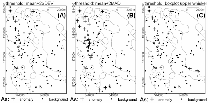
Fig. 3-17. Anomalies in the log
e
-transformed As data subsets according to rock type at sample
points and exclusive of As censored values (see Table 3-IV), Aroroy district (Philippines).
Anomalies are based on threshold defined as (A) mean+2SDEV, (B) median+2MAD and (C)
boxplot UW. Triangles represent locations of epithermal Au deposit occurrences. Light-grey lines
represent lithologic contacts (see Fig. 3-9).

76 Chapter 3
associations reflecting presence of epithermal Au deposits. Such questions can be
answered by application of bivariate analytical techniques.
Scatterplots are useful for visual exploration of inter-element relationships.
Scatterplots of raw or transformed data inclusive of samples with censored values (Figs.
3-18A and 3-18C) lead to misguided interpretations about inter-element relationships.
Scatterplots of raw data exclusive of samples with censored values (Fig. 3-18B) also lead
to misguided interpretations about inter-element relationships. Obvious data outliers
(say, based on boxplots) must also be removed in creating scatterplots. The As outliers
recognised in the uni-element data analyses are obvious in the scatterplots of the raw
data (Figs. 3-18A and 3-18B) but not in the scatterplots of the log
e
-transformed data
(Figs. 3-18C and 3-18D). Thus, transformation of data values (so that they approach
symmetrical distributions) and removal of samples with censored values result in
Fig. 3-18. Scatterplots of the uni-element data sets, Aroroy district (Philippines). (A) Raw data.
(B) Raw data exclusive of samples with censored As values. (C) Log
e
-transformed (ln) data. (D)
Log
e
-transformed (ln) data exclusive of samples with censored As values.

Exploratory Analysis of Geochemical Anomalies 77
scatterplots that are optimal for visual analysis of inter-element relationships. The
scatterplots in Fig. 3-18D indicate that all the elements under study have positive
relationships with each other and there is no obvious presence of more than one
population, except for a small cluster of high Mn values and low As values in the Mn-As
plot. This small cluster in the Mn-As plot pertains to 13 samples in areas underlain by
diorite with As concentrations above detection limit (see Table 3-II or 3-IV)).
Visual interpretation of a scatterplot can be aided by estimation of correlation
coefficients and of covariance values between two uni-element data sets to obtain
impressions about, respectively, inter-relation of data values and mutual variability of
values. Estimates of correlation coefficients and covariance values are affected by data
form and presence of censored values, outliers and multiple populations. The correlation
coefficients and covariance values of element pairs corresponding to the data scatterplots
in Fig. 3-18D are shown in Tables 3-V and 3-VI, respectively. Statistically significant
positive correlations exist between all pairs of the log
e
-transformed uni-element data sets
exclusive of samples with censored As values. The strongest correlation is between Ni
and Co, followed by inter-element correlations with Mn. These correlations suggest
controls by either lithology or scavenging by Mn-oxides. From the estimated correlation
coefficients (Table 3-V), there are no obvious inter-element relationships reflecting
presence of mineralisation. Estimates of covariance values for each pair of the uni-
TABLE 3-V
Correlations coefficients of the log
e
-transformed uni-element data exclusive of samples with
censored As values (n=95), Aroroy district (Philippines).
Cu Zn Ni Co Mn
Zn 0.342
Ni 0.560 0.537
Co 0.396 0.589 0.754
Mn 0.268 0.730 0.440 0.661
As 0.341 0.414 0.496 0.391 0.462
All coefficients are si
g
nificant at the 0.01
p
robabilit
y
level
(
2-tailed test
)
.
TABLE 3-VI
Covariance matrix of the log
e
-transformed uni-element data exclusive of samples with censored As
values (n=95), Aroroy district (Philippines).
Cu Zn Ni Co Mn
Zn 0.091
Ni 0.188 0.135
Co 0.104 0.115 0.187
Mn 0.066 0.134 0.103 0.120
As 0.237 0.214 0.326 0.200 0.222
78 Chapter 3
element data sets (Table 3-VI), nevertheless, indicate a Cu-Ni-Co association reflecting
lithologic control, a Mn-Zn-Co association reflecting metal scavenging chemical control
by Mn-oxides and an As-Ni-Cu association reflecting metallic mineralisation related to
certain lithologies (i.e., andesitic rather than dacitic). The presence of obvious and subtle
inter-element relationships in the case study data sets requires further application of
appropriate multivariate methods that allow quantification and mapping of such inter-
element relationships.
Analysis and mapping of multi-element associations
The multivariate methods most commonly employed in studying and quantifying
multi-element associations in exploration geochemical data include principal
components analysis (PCA), factor analysis (FA), cluster analysis (CA), regression
analysis (RA) and discriminant analysis (DA). PCA and FA are useful in studying inter-
element relationships hidden in multiple uni-element data sets. CA is useful for studying
inter-sample relationships, whilst RA and DA are useful for studying inter-element as
well as inter-sample associations. RA and DA require training data, i.e., samples
representative of processes of interest (e.g., from mineralised zones). Authoritative
explanations of multivariate methods applied to geochemical and geological data
analysis can be found in Howarth and Sinding-Larsen (1983) and Davis (2002). In this
case study, either PCA or FA is favourable for revealing inter-element relationships, a
few of which may reflect presence of mineralisation.
PCA and FA are very similar techniques so that they are often confused with each
other, but they have significant mathematical and conceptual differences. Howarth and
Sinding-Larsen (1983) and Reimann et al. (2002) provide clear discussions about the
similarities and dissimilarities between PCA and FA, which are summarised here. Both
methods start with either the correlation matrix or the covariance matrix of data for a
number (n) of variables. Both of them require transformation and/or standardisation of
the input data. The main difference between PCA and FA is related to the proportions of
the total variance of data for n variables accounted for in the analysis. The total variance
is composed of the common variance in all n variables and the specific variances of each
of the n
th
variable. In PCA, principal components (or PCs) are determined, without any
statistical assumptions, to account for the maximum total variance of all input variables.
In FA, a number of common factors are defined, with assumption of a statistical model
with certain prerequisites, to account maximally for the common inter-correlation
between the input variables. Thus, on the one hand, PCA is variance-oriented and results
in a number of uncorrelated PCs (equal to n input variables) that altogether account for
the total variance of all input variables. The 1
st
PC accounts for the highest proportion of
the total variance (and thus represents the ‘most common’ variance) of the multivariate
data, whereas the n
th
(or last) PC accounts for the least proportion of the total variance
(and thus represents the ‘most specific’ variance) of the multivariate data. On the other
hand, FA is correlation-oriented and results in a number (k) of uncorrelated common
factors (less than the n input variables) that together do not account for the total variance
of all input variables but altogether account for maximum common variance in all the
Exploratory Analysis of Geochemical Anomalies 79
input variables. Thus, the first factor accounts for the highest proportion of the ‘total’
common variance in the input multivariate data, whereas the k
th
(or last) factor accounts
for the least proportion of the ‘total’ common variance in the input multivariate data.
Because the ‘total’ common variance in n input multivariate data is unknown, the
‘optimum’ k common factors must be determined by following a number of statistical
tests (Basilevsky, 1994) or ‘rule-of-thumb’ criteria, e.g., factors that cumulatively
account for at least 70% of the total variance (Reimann et al., 2002). From the foregoing
discussion, the following can be said about the applicability of either PCA or FA in
geochemical data analysis (cf. Howarth and Sinding-Larsen, 1983). On the one hand,
PCA is favourable in cases of geochemical data analysis in which the range of PCs
representing the ‘most common’ variance to the ‘most specific’ variance in the input
multi-element data sets is of interest to allow recognition of latent inter-element
variations that reflect the various geochemical processes in a study area. On the other
hand, FA is favourable in cases of geochemical data analysis in which the factors
representing the ‘most common’ variance in the input multi-element data sets are of
interest to allow recognition of latent inter-element relationships that describe the
different geochemical processes in a study area.
Therefore, based on the preceding discussion about the difference between PCA and
FA, the former is considered more appropriate to apply in the case study than the latter
because of its ‘exploratory’ rather than ‘confirmatory’ nature. In PCA, it is essential to
use standardised data if the correlation matrix is used to derive the PCs or to use
unstandardised data if the covariance matrix is used to derive the PCs (Trochimczyk and
Chayes, 1978). In addition, because estimates of either the correlation coefficient or the
covariance are influenced by data form, presence of censored values, outliers and more
than one population, it is also essential to ‘clean’ and transform the data so that they
approach a (nearly) symmetrical distribution. For the same log
e
-transformed uni-element
data sets that were used to create the scatterplots in Fig. 3-18D, the correlation matrix in
Table 3-V and the covariance matrix in Table 3-VI, the derived PCs are shown in Table
3-VII. The correlation matrix (Table 3-V) was used to derive the PCs, so the uni-element
data sets were first standardised using equation (3.11).
In Table 3-VII, the first two PCs (PC1 and PC2) together explain the ‘most common’
variance in the multivariate data and thus represent multi-element associations that
reflect the major geochemical processes in the study area. PC1 accounts for at least 58%
of the total variance and represents a Co-Ni-Zn-Mn-As-Cu association, which reflects a
plausible combination (or overprinting) of lithologic and chemical controls. PC2
explains about 15% of the total variance and represents two antipathetic associations – a
Cu-Ni association reflecting lithologic control and a Mn-Zn association reflecting metal
scavenging control by Mn-oxides. Each of the last four PCs (PC3-PC6) explains the
specific variances in the multivariate data and represents multi-element associations that
reflect either the minor (or subtle) geochemical processes in the study area or errors in
the multivariate data. PC3 accounts for at least 11% of the total variance and represents
two antipathetic associations – an As-dominated multi-element association reflecting
mineralisation control and a Co-Ni association reflecting lithologic control. The last