Devore J.L., Berk K.N. Modern Mathematical Statistics with Applications

Подождите немного. Документ загружается.

mðm þ 2n þ 1Þ=2. As with the special case m ¼ 3, n ¼ 4, the distribution of W is

symmetric about the value that is halfway between the smallest and largest values;

this middle value is m(m + n + 1)/2. Because of this symmetry, probabilities

involving lower-tail critical values can be obtained from corresponding upper-tail

values.

Null hypothesis: H

: m

 m

¼ D

Test statistic value : w ¼

i¼1

where r

¼ rank of ðx

 D

Þ in the

combined sample of m þ n ðx  D

Þ’s

and y’s

Alternative Hypothesis Rejection Region

: m

 m

> D

w  c

: m

 m

< D

w  mðm þ n þ 1Þc

: m

 m

6¼ D

either w  c or w  mðm þ n þ 1Þc

where P(W  c

when H

is true)  a, P(W  c when H

is true)  a/2.

Because W has a discrete probability distribution, there will not always exist

a critical value corresponding exactly to one of the usual levels of significance.

Appendix Table A.13 gives upper-tail critical values for probabilities closest to .05,

.025, .01, and .005, from which level .05 or .01 one- and two-tailed tests can be

obtained. The table gives information only for m ¼ 3, 4, ..., 8 and n ¼ m, m +1,

... , 8 (i.e., 3  m  n  8). For values of m and n that exceed 8, a normal

approximation can be used (Exercise 14). To use the table for small m and n,

though, the X and Y samples should be labeled so that m  n.

Example 14.3 The urinary fluoride conce ntration (parts per million) was measured both for a

sample of livestock grazing in an area previously exposed to fluoride pollution and

for a similar sample grazing in an unpolluted region:

Polluted 21.3 18.7 23.0 17.1 16.8 20.9 19.7

Unpolluted 14.2 18.3 17.2 18.4 20.0

Does the data indicate strongly that the true average fluoride concentration for

livestock grazing in the polluted region is larger than for the unpolluted region? Use

the Wilcoxon rank-sum test at level a ¼ .01.

The sample sizes here are 7 and 5. To obtain m  n, label the unpolluted

observations as the x’s (x

¼ 14.2, ... , x

¼ 20.0) and the polluted observations

as the y ’s. Thus m

is the true average fluoride concentration without pollution, and

is the true average concentration with pollution. The alternative hypothesis is

: m

 m

< 0 (pollution causes an increase in concentration), so a lower-tailed

768 CHAPTER 14 Alternative Approaches to Inference

test is appropriate. From Appendix Table A.13 with m ¼ 5 and n ¼ 7, P(W  47

when H

is true)  .01. The critical value for the lower-tailed test is therefore

m(m + n +1) 47 ¼ 5(13)  47 ¼ 18; H

will now be rejected if w  18.

The pooled ordered sample follows; the computed W is w ¼ r

þ r

þþr

(where r

is the rank of x

) ¼ 1+5+4+6+9¼ 25. Since 25 is not  18, H

not rejected at (approximately) level .01.

xyyxxxyyxyyy

14.2 16.8 17.1 17.2 18.3 18.4 18.7 19.7 20.0 20.9 21.3 23.0

123456789101112

■

Ties are handled as suggested for the signed-rank test in the previous section.

Efﬁciency of the Wilcoxon Rank-Sum Test

When the distributions being sampled are both normal with s

¼ s

, and therefore

have the same shapes and spreads, either the pooled t test or the Wilcoxon test can

be used (th e two-sample t test assumes normality but not equal variances, so

assumptions underlying its use are more restrictive in one sense and less in another

than those for Wilcoxon’s test). In this situation, the pooled t test is best among all

possible tests in the sense of minimizing b for any fixed a. However, an investigator

can never be absolutely certain that underlying assumptions are satisfied. It is

therefore relevant to ask (1) how much is lost by using Wilcoxon’s test rather

than the pooled t test when the distributions are normal with equal variances and

(2) how W compares to T in nonnormal situations.

The notion of test efficiency was discussed in the previous section in connec-

tion with the one-sample t test and Wilcoxon signed-rank test. The results for the

two-sample tests are the same as those for the one-sample tests. When normality

and equal variances both hold, the rank-sum test is approximately 95% as efficient

as the pooled t test in large samples. That is, the t test will give the same error

probabilities as the Wilcoxon test using slightly smaller sample sizes. On the other

hand, the Wilcoxon test will always be at least 86% as efficient as the pooled t test

and may be much more efficient if the underlying distributions are very nonnormal,

especially with heavy tails. The com parison of the Wilcoxon test with the two-

sample (unpooled) t test is less clear-cut. The t test is not known to be the best test in

any sense, so it seems safe to conclude that as long as the population distributions

have similar shapes and spreads, the behavior of the Wilcoxon test should compare

quite favorably to the two-sample t test.

Lastly, we note that b calculat ions for the Wilcoxon test are quite difficult.

This is because the distribution of W when H

is false depends not only on m

 m

but also on the shapes of the two distributions. For most underlying distributions,

the nonnull distribution of W is virtually intractable. This is why statisticians have

developed large-sample (asymptotic relative) efficiency as a means of comparing

tests. With the capabilities of modern-day computer software, another approach to

calculation of b is to carry out a simulation experiment.

14.2 The Wilcoxon Rank-Sum Test 769

Exercises Section 14.2 (9–16)

9. In an experiment to compare the bond strength of

two different adhesives, each adhesive was used in

five bondings of two surfaces, and the force nec-

essary to separate the surfaces was determined for

each bonding. For adhesive 1, the resulting values

were 229, 286, 245, 299, and 250, whereas the

adhesive 2 observations were 213, 179, 163, 247,

and 225. Let m

denote the true average bond

strength of adhesive type i. Use the Wilcoxon

rank-sum test at level .05 to test H

: m

¼ m

versus H

: m

> m

10. The article “A Study of Wood Stove Particulate

Emissions” (J. Air Pollut. Contr. Assoc., 1979:

724–728) reports the following data on burn time

(hours) for samples of oak and pine. Test at level

.05 to see whether there is any difference in true

average burn time for the two types of wood.

Oak 1.72 .67 1.55 1.56 1.42 1.23 1.77 .48

Pine .98 1.40 1.33 1.52 .73 1.20

11. A modification has been made to the process for

producing a certain type of “time-zero” film (film

that begins to develop as soon as a picture is taken).

Because the modification involves extra cost, it will

be incorporated only if sample data strongly indi-

cates that the modification has decreased true aver-

age developing time by more than 1 s. Assuming

that the developing-time distributions differ only

with respect to location if at all, use the Wilcoxon

rank-sum test at level .05 on the accompanying data

to test the appropriate hypotheses.

Original

Process 8.6 5.1 4.5 5.4 6.3 6.6 5.7 8.5

Modified

Process 5.5 4.0 3.8 6.0 5.8 4.9 7.0 5.7

12. The article “Measuring the Exposure of Infants to

Tobacco Smoke” (New Engl. J. Med., 1984:

1075–1078) reports on a study in which various

measurements were taken both from a random

sample of infants who had been exposed to house-

hold smoke and from a sample of unexposed

infants. The accompanying data consists of obser-

vations on urinary concentration of cotinine, a

major metabolite of nicotine (the values constitute

a subset of the original data and were read from a

plot that appeared in the article). Does the data

suggest that true average cotinine level is higher in

exposed infants than in unexposed infants by more

than 25? Carry out a test at significance level .05.

Unexposed 81112142043111

Exposed 35 56 83 92 128 150 176 208

13. Reconsider the situation described in Exercise 100

of Chapter 10 and the accompanying MINITAB

output (the Greek letter eta is used to denote a

median).

Mann-Whitney Confidence Interval and

Test

good N

¼ 8 Median ¼ 0.540

poor N

¼ 8 Median ¼ 2.400

Point estimate for ETA1

 ETA2 is

1.155

95.9 % CI for ETA1  ETA2 is(  3.160,

0.409) W ¼ 41.0

Test of ETA1

¼ ETA2 vs ETA1 < ETA2 is

significant at 0.0027

a. Verify that the value of MINITAB’s test statis-

tic is correct.

b. Carry out an appropriate test of hypotheses

using a significance level of .01.

14. The Wilcoxon rank-sum statistic can be repre-

sented as W ¼ R

þ R

þþR

, where R

the rank of X

 D

among all m + n such differ-

ences. When H

is true, each R

is equally likely to

be one of the first m + n positive integers; that is,

has a discrete uniform distribution on the values

1, 2, 3, ..., m + n.

a. Determine the mean value of each R

when H

is true and then show that the mean value of W

is m(m+n+1)/2. [Hint: Use the hint given in

Exercise 6(a).]

b. The variance of each R

is easily determined.

However, the R

’s are not independent random

variables because, for example, if m ¼ n ¼ 10

and we are told that R

¼ 5, then R

must

be one of the other 19 integers between 1

and 20. However, if a and b are any two

distinct positive integers between 1 and

m+n inclusive, it follows that

PðR

¼ a and R

¼ bÞ¼1=½ðm þ nÞðm þ n  1Þ

since two integers are being sampled without

replacement from among 1, 2,

... , m+n.

Use this fact to show that

CovðR

; R

Þ¼

ðm þ n þ 1Þ=12

and then show that the vari-

ance of W is

mnðm þ n þ 1Þ=12.

c. A central limit theorem for a sum of non-inde-

pendent variables can be used to show that

when m > 8 and n > 8, W has approximately

a normal distribution with mean and variance

given by the results of (a) and (b). Use this to

770

CHAPTER 14 Alternative Approaches to Inference

propose a large-sample standardized rank-sum

test statistic and then describe the rejection

region that has approximate significance level

a for testing H

against each of the three

commonly encountered alternative hypotheses.

[Note: When there are ties in the observed

values, a correction for the variance derived

in (b) should be used in standardizing W; please

consult a book on nonparametric statistics for

the result.]

15. The accompanying data resulted from an experi-

ment to compare the effects of vitamin C in orange

juice and in synthetic ascorbic acid on the length

of odontoblasts in guinea pigs over a 6-week

period (“The Growth of the Odontoblasts of the

Incisor Tooth as a Criterion of the Vitamin C

Intake of the Guinea Pig,” J. Nutrit., 1947:

491–504). Use the Wilcoxon rank-sum test at

level .01 to decide whether true average length

differs for the two types of vitamin C intake.

Compute also an approximate P-value. [Hint:

See Exercise 14.]

Orange Juice 8.2 9.4 9.6 9.7 10.0 14.5

15.2 16.1 17.6 21.5

Ascorbic Acid 4.2 5.2 5.8 6.4 7.0 7.3

10.1 11.2 11.3 11.5

16. Test the hypotheses suggested in Exercise 15

using the following data:

Orange Juice 8.2 9.5 9.5 9.7 10.0 14.5

15.2 16.1 17.6 21.5

Ascorbic Acid 4.2 5.2 5.8 6.4 7.0 7.3

9.5 10.0 11.5 11.5

[Hint: See Exercise 14.]

14.3

Distribution-Free Confidence Intervals

The method we have used so far to construct a confidence interval (CI) can be

described as follows: Start with a random variable (Z, T, w

, F, or the like) that

depends on the parameter of interest and a probability statement involving the

variable, manipulate the inequalities of the statement to isolate the parameter

between random endpoints, and finally substitute computed values for random

variables. Another general method for obtaining CIs takes advantage of a relation-

ship between test procedures and CIs. A 100(1  a)% CI for a parameter y can be

obtained from a level a test for H

: y ¼ y

versus H

: y 6¼ y

. This method will

be used to derive intervals associated with the Wilcoxon signed-rank test and the

Wilcoxon rank-sum test.

Before using the method to derive new intervals, reconsider the t test and the

t interval. Suppose a random sample of n ¼ 25 observations from a normal

population yields summary statistics

x¼ 100, s ¼ 20. Then a 90% CI for m is

x  t

:05;24



ﬃﬃﬃﬃﬃ

;

x þ t

:05;24



ﬃﬃﬃﬃﬃ



¼ð93 :16; 106:84Þð14: 2 Þ

Suppose that instead of a CI, we had wished to test a hypoth esis about m. For

: m ¼ m

versus H

: m 6¼ m

, the t test at level .10 specifies that H

should be

rejected if t is either  1.711 or 1.711, where

t ¼

x  m

ﬃﬃﬃﬃﬃ

100  m

20=

ﬃﬃﬃﬃﬃ

100  m

ð14:3Þ

Consider now the null value m

¼ 95. Then t ¼ 1.25, so H

is not rejected.

Similarly, if m

¼ 104, then t ¼1, so again H

is not rejected. However,

if m

¼ 90, then t ¼ 2.5, so H

is rejected, and if m

¼ 108, then t ¼2, so H

is again rejected. By considering other values of m

and the decision resulting

from each one, the following general fact emerges: Every number inside the

14.3 Distribution-Free Conﬁdence Intervals 771

interval (14.2) specifies a value of m

for which t of (14.3) leads to nonrejection of

, whereas every number outside interval (14.2) corresponds to a t for which H

rejected. That is, for the fixed values of n,

x, and s, the interval (14.2) is precisely

the set of all m

values for which testing H

: m ¼ m

versus H

: m 6¼ m

results in

not rejecting H

PROPOSITION

Suppose we have a level a test procedure for testing H

: y ¼ y

versus

: y 6¼ y

. For fixed sample values, let A denote the set of all values

for which H

is not rejected. Then A is a 100(1  a)% CI for y.

There are actually pathological examples in which the set A defined in the

proposition is not an interval of y values, but instead the complement of an interval

or something even stranger. To be more precise, we should reall y replace the notion

of a CI with that of a confidence set. In the cases of interest here, the set A does

turn out to be an interval.

The Wilcoxon Signed-Rank Interval

To test H

: m ¼ m

versus H

: m 6¼ m

using the Wilcoxon signed-rank test, where

m is the mean of a continuous symmetric distribution, the absolute values

 m

; ...;

 m

j are ordered from smallest to largest, with the smallest

receiving rank 1 and the largest, rank n. Each rank is then given the sign of its

associated x

 m

, and the test statistic is the sum of the positively signed ranks.

The two-tailed test rejects H

if s

is either  c or  n(n + 1)/2  c, where c is

obtained from Appendix Table A.12 once the desired level of significance a is

specified. For fixed x

, ..., x

, the 100(1  a)% signed-rank interval will consist of

all m

for which H

: m ¼ m

is not rejected at level a. To identify this interval, it is

convenient to express the test statistic S

in another form.

¼ the number of pairwise averages X

þ X



=2 with i  j

that are  m

ð14:4Þ

That is, if we average each x

in the list with each x

to its left, including (x

+ x

)/2

(which is just x

), and count the number of these averages that are  m

, s

results.

In moving from left to right in the list of sample values, we are simply averaging

every pair of observations in the sample [again including (x

+ x

)/2] exactly once,

so the order in which the observations are listed before averaging is not important.

The equivalence of the two methods for computing s

is not difficult to verify. The

number of pairwise averages is



þ n (the first term due to averaging of different

observations and the second due to averaging each x

with itself), which equals

n(n + 1)/2. If either too many or too few of these pairwise averages are  m

is rejected.

772 CHAPTER 14 Alternative Approaches to Inference

Example 14.4 The following observations are values of cerebral metabolic rate for rhesus monkeys:

¼ 4.51, x

¼ 4.59, x

¼ 4.90, x

¼ 4.93, x

¼ 6.80, x

¼ 5.08, x

¼ 5.67. The

28 pairwise averages are, in increasing order,

4.51 4.55 4.59 4.705 4.72 4.745 4.76 4.795 4.835 4.90

4.915 4.93 4.99 5.005 5.08 5.09 5.13 5.285 5.30 5.375

5.655 5.67 5.695 5.85 5.865 5.94 6.235 6.80

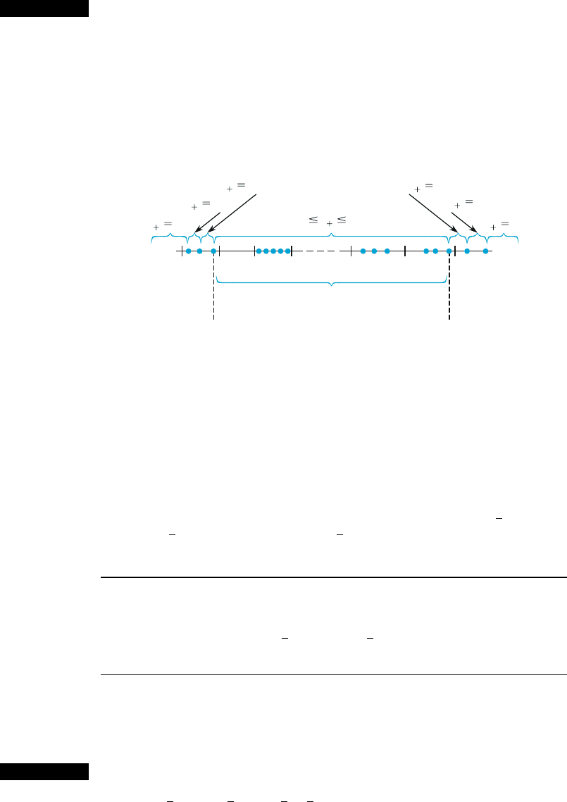
The first few and the last few of these are pictured on a measurement axis in Figure 14.2.

Because of the discreteness of the distribution of S

, a ¼ .05 cannot be

obtained exactly. The rejection region {0, 1, 2, 26, 27, 28} has a ¼ .046, which

is as close as possible to .05, so the level is approximately .05. Thus if the number of

pairwise averages  m

is between 3 and 25, inclusive, H

is not rejected. From

Figure 14.2 the (approximate) 95% CI for m is (4.59, 5.94).

■

In general, once the pairwise averages are ordered from smallest to largest,

the endpoints of the Wilcoxon interval are two of the “extreme” averages. To

express this precisely, let the smallest pairwise average be denoted by

ð1Þ

, the next

smallest by

ð2Þ

; ... ; and the largest by x

ðnðnþ1Þ=2Þ

PROPOSITION

If the level a Wilcoxon signed-rank test for H

: m ¼ m

versus H

: m 6¼ m

is to

reject H

if either s

 c or s

 n(n +1)/2 c, then a 100(1  a)% CI for m is

ðnðnþ1Þ=2cþ1Þ

; x

ðcÞ

Þð14:5Þ

In words, the interval extends from the dth smallest pairwise average to the dth

largest average, where d ¼ nðn þ 1Þ=2  c þ 1. Appendix Table A.14 gives the

values of c that correspond to the usual confidence levels for n ¼ 5, 6, ... , 25.

Example 14.5

(Example 14.4

continued)

For n ¼ 7, an 89.1% interval (approximately 90%) is obtained by using c ¼ 24

(since the rejection region {0, 1, 2, 3, 4, 24, 25, 26, 27, 28} has a ¼ .109). The

interval is ð

ð2824þ1Þ

; x

ð24Þ

Þ¼ðx

ð5Þ

; x

ð24Þ

Þ¼ 4:72; 5:85ðÞ, which extends from the

fifth smallest to the fifth largest pairwise average.

■

At level .0469, H

not rejected for m

in here

4.8 5.5 5.75 64.5 4.6 4.7

s 2

3 s 25

Figure 14.2 Plot of the data for Example 14.4

14.3 Distribution-Free Conﬁdence Intervals 773

The derivation of the interval depended on having a single sample from a continuous

symmetric distribution with mean (median) m. When the data is paired, the interval

constructed from the differences d

, d

, ... , d

is a CI for the mean (median)

difference m

. In this case, the symmetry of X and Y distributions need not be

assumed; as long as the X and Y distributions have the same shape, the X  Y

distribution will be symmetric, so only continuity is required.

For n > 20, the large-sample approximat ion (Exercise 6) to the Wilcoxon

test based on standardizing S

gives an approximation to c in (14.5). The result

[for a 100(1  a)% interval] is

c 

nðn þ 1Þ

þ z

a=2

ﬃﬃﬃﬃﬃﬃﬃﬃﬃﬃﬃﬃﬃﬃﬃﬃﬃﬃﬃﬃﬃﬃﬃﬃﬃﬃﬃﬃﬃﬃﬃﬃﬃﬃ

nðn þ 1Þð2n þ 1Þ

The efficiency of the Wilcoxon interval relative to the t interval is roughly the

same as that for the Wilcoxon test relative to the t test. In particular, for large

samples when the underlying population is normal, the Wilcoxon interval will tend

to be slightly longer than the t interval, but if the population is quite nonnormal

(symmetric but with heavy tails), then the Wilcoxon interval will tend to be

much shorter than the t interval. And as we emphasized earlier in our discussion

of bootstrapping, in the pres ence of nonnormality the actual confidence level of

the t interval may differ considerably from the nominal (e.g., 95%) level.

The Wilcoxon Rank-Sum Interval

The Wilcoxon rank-sum test for testing H

: m

 m

¼ D

is carried out by first

combining the (X

 D

)’s and Y

’s into one sample of size m + n and ranking them

from smallest (rank 1) to largest (rank m + n). The test statistic W is then the sum of

the ranks of the (X

 D

)’s. For the two-sided alternative, H

is rejected if w is

either too small or too large.

To obtain the associated CI for fixed x

’s and y

’s, we must d eter mine the set

of all D

values for which H

is not rej ected. This is easiest to do if we first express

the test statistic in a slightly different form. The smallest possible value of W is

m(m + 1)/2, corresponding to every (X

 D

)lessthaneveryY

,andtherearemn

differences of the form (X

 D

)  Y

. A bit of manipulation gives

W ¼½number of (X

 Y

 D

Þ’s  0þ

mðm þ 1Þ

¼½number o f (X

 Y

Þ’s  D

þ

mðm þ 1Þ

ð14:6Þ

Thus rejecting H

if the number of (x

 y

)’s  D

is either too small or too large

is equivalent to rejecting H

for small or large w.

Expression (14.6) suggests that we compute x

 y

for each i and j and order

these mn differences from smallest to largest. Then if the null value D

is neither

smaller than most of the differences nor larger than most, H

: m

 m

¼ D

is not

rejected. Varying D

now shows that a CI for m

 m

will have as its lower

endpoint one of the ordered (x

 y

)’s, and similarly for the upper endpoint.

774 CHAPTER 14 Alternative Approaches to Inference

PROPOSITION

Let x

, ..., x

and y

, ..., y

be the observed values in two independent samples

from continuous distributions that differ only in location (and not in shape).

With d

¼ x

 y

and the ordered differences denoted by d

ij(1)

, d

ij(2)

, ..., d

ij(mn)

the general form of a 100(1  a)% CI for m

 m

ðd

ijðmncþ1Þ

; d

ijðcÞ

Þð14:7Þ

where c is the critical constant for the two-tailed level a Wilcoxon rank-sum test.

Notice that the form of the Wilcoxon rank-sum interval (14.7) is very similar to the

Wilcoxon signed-rank interval (14.5); (14.5) uses pairwise averages from a single

sample, whereas (14.7) uses pairwise differences from two samples. Appendix

Table A.15 gives values of c for selected values of m and n.

Example 14.6 The article “Some Mechanical Properties of Impregnated Bark Board” (Forest

Products J., 1977: 31–38) reports the following data on maximum crushing strength

(psi) for a sample of epoxy-impregnated bark board and for a sample of bark board

impregnated with another polymer:

Epoxy (x’s) 10,860 11,120 11,340 12,130 14,380 13,070

Other (y’s) 4,590 4,850 6,510 5,640 6,390

Obtain a 95% CI for the true average difference in crushing strength between the

epoxy-impregnated board and the other type of board.

From Appendix Table A.15, since the smaller sample size is 5 and the larger

sample size is 6, c ¼ 26 for a confidence level of approximately 95%. The d

’s

appear in Table 14.4. The five smallest d

’s [d

ij(1)

, ..., d

ij(5)

] are 4350, 4470, 4610,

4730, and 4830; and the five largest d

’s are (in descending order) 9790, 9530,

8740, 8480, and 8220. Thus the CI is (d

ij(5)

, d

ij(26)

) ¼ (4830, 8220).

■

When m and n are both large, the Wilcoxon test statistic has approximately a

normal distribution (Exer cise 14). This can be used to derive a large-sample

approximation for the value c in interval (14.7). The result is

Table 14.4 Differences (d

) for the rank-sum interval in Example 14.6

4590 4850 5640 6390 6510

10,860 6270 6010 5220 4470 4350

11,120 6530 6270 5480 4730 4610

11,340 6750 6490 5700 4950 4830

12,130 7540 7280 6490 5740 5620

13,070 8480 8220 7430 6680 6560

14,380 9790 9530 8740 7990 7870

14.3 Distribution-Free Conﬁdence Intervals 775

c 

þ z

a=2

ﬃﬃﬃﬃﬃﬃﬃﬃﬃﬃﬃﬃﬃﬃﬃﬃﬃﬃﬃﬃﬃﬃﬃﬃﬃﬃﬃﬃﬃﬃ

mnðm þ n þ 1Þ

ð14:8Þ

As with the signed-rank interval, the rank-sum interval (14.7) is quite effi-

cient with respect to the t interval; in large samples, (14.7) will tend to be only a bit

longer than the t interval when the underlying populations are normal and may be

considerably shorter than the t interval if the underlying populations have heavier

tails than do norm al populations. And once again, the actual confidence level for

the t interval may be quite different from the nominal level in the presence of

substantial nonnormality.

Exercises Section 14.3 (17–22)

17. The article “The Lead Content and Acidity of

Christchurch Precipitation” (New Zeal. J. Sci.,

1980: 311–312) reports the accompanying data

on lead concentration (mg/L) in samples gathered

during eight different summer rainfalls: 17.0,

21.4, 30.6, 5.0, 12.2, 11.8, 17.3, and 18.8. Assum-

ing that the lead-content distribution is symmetric,

use the Wilcoxon signed-rank interval to obtain a

95% CI for m.

18. Compute the 99% signed-rank interval for true

average pH m (assuming symmetry) using the

data in Exercise 3. [Hint: Try to compute only

those pairwise averages having relatively small

or large values (rather than all 105 averages).]

19. Compute a CI for m

of Example 14.2 using the

data given there; your confidence level should be

roughly 95%.

20. The following observations are amounts of hydro-

carbon emissions resulting from road wear of bias-

belted tires under a 522-kg load inflated at

228 kPa and driven at 64 km/h for 6 h (“Charac-

terization of Tire Emissions Using an Indoor Test

Facility,” Rubber Chem. Tech., 1978: 7–25): .045,

.117, .062, and .072. What confidence levels are

achievable for this sample size using the signed-

rank interval? Select an appropriate confidence

level and compute the interval.

21. Compute the 90% rank-sum CI for m

 m

using

the data in Exercise 9.

22. Compute a 99% CI for m

 m

using the data in

Exercise 10.

14.4

Bayesian Methods

Consider making an inference about some parameter y. The “frequentist” or

“classical” approach, which we have followed until now in this book, is to regard

the value of y as fixed but unknown, observe data from a joint pmf or pdf

f ð x

; ...; x

; yÞ, and use the observations to draw appropriate conclusions. The

Bayesian or “subjective” paradigm is different. Again the value of y is unknown,

but Bayesians say that all available information about it—intuition, data from past

experiments, expert opinions , etc. —can be incorporated into a prior distribution,

usually a prior pdf g(y) since there will typically be a continuum of possible values

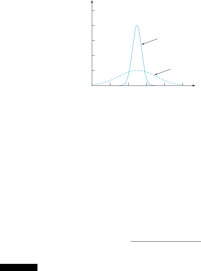
of the parameter rather than just a discrete set. If there is substantial knowledge

about y, the prior will be quite peaked and highly concentrated about some central

value, whereas a lack of information is shown by a relatively flat “uninformative”

prior. These possibilities are illustrated in Figure 14.3.

In esse nce we are now thinking of the actual value of y as the observed value

of a random variable Y, although unfortun ately we ourselves don’t get to observe

the value. The (prior) distribution of this random variable is g(y). Now, just as in

776 CHAPTER 14 Alternative Approaches to Inference

the frequentist scenario, an experiment is performed to obtain data. The joint pmf or

pdf of the data given the value of y is pðx

; ...; x

jyÞ or f ðx

; ...; x

jyÞ. We use a

vertical line segment here rather than the earlier semicolon to emphasize that we are

conditioning on the value of a random variable.

At this point, an appropriate version of Bayes’ theorem is used to obtain

h(yjx

,...,x

), the posterior distribution of the parameter. In the Bayesian world,

this posterior distribution contains all current information about y. In particular, the

mean of this posterior distribution gives a point estimate of the parameter.

An interval [a, b] having posterior probability .95 gives a 95% credibility interval,

the Bayesian analogue of a 95% confidence interval (but the interpretation is

different). After presenting the necessary version of Bayes’ Theorem, we illustrate

the Bayesian approach with two examples.

Bayes’ theorem here needs to be a bit more general than in Section 2.4 to

allow for the possibility of continuous distributions. This version gives the posterior

distribution h(y | x

, ...,x

) as a product of the prior pdf times the conditional

pdf, with a denominator to assure that the total posterior probability is 1:

hðyjx

; x

; ...; x

Þ¼

f ð x

; x

; ...; x

jyÞgðyÞ

1

f ð x

; x

; ...; x

jyÞgðyÞdy

Example 14.7 Suppose we want to make an inference about a population proportion p. Since the

value of this parameter must be between 0 and 1, and the family of standard beta

distributions is concentrated on the interval [0, 1], a particular beta distribution is a

natural choice for a prior on p. In particular, consider data from a survey of 1574

American adults reported by the National Science Foundation in May 2002.

Of those responding, 803 (51%) incorrectly said that antibiotics kill viruses.

In accord with the discussi on in Section 3.5, the data can be considered either a

random sample of 1574 from the Bernoulli distribution (binomial with number of

trials ¼ 1) or a single observation from the binomial distribution with n ¼ 1574.

We use the latter approach here, but Exercise 23 involves showing that the

Bernoulli approach is equivalent.

0.2

0.0

0.8

0.6

0.4

1.0

0246810

Prior pdf

Wide

Narrow

Figure 14.3 A narrow concentrated prior and a wider less informative prior

14.4 Bayesian Methods 777