Egerton R.F. Electron Energy-Loss Spectroscopy in the Electron Microscope
Подождите немного. Документ загружается.

48 2 Energy-Loss Instrumentation
Second, the focusing power in the axial (y-) direction is decreased, whereas the
radial (x-) focusing remains practically unaltered. As a result, either ε
1
or ε
2
must be
increased (compared to the SCOFF prediction) in order to maintain double focusing.
The net result is a slight increase in image distance; see Fig. 2.8.
A third effect of the extended fringing fields is to add a convex component of
curvature to the entrance and exit edges of the magnet, the magnitude of this com-
ponent varying inversely with the polepiece width w. Such curvature affects the
spectrometer aberrations, as discussed in Section 2.2.2. Finally, the extended fring-
ing field introduces a discrepancy between the “effective” edge of the magnet (which
serves as a reference point for measuring object and image distances) and the actual
“mechanical” edge, the former generally lying outside the latter.
To define the spatial extent of the fringing field, so that it can be properly taken
into account in EFF calculations and is less affected by the surroundings of the
spectrometer, plates made of a soft magnetic material (“mirror planes”) are some-
times placed parallel to the entrance and exit edges, to “clamp” the field to a low
value at the required distance from the edge. If the plate–polepiece separation is
chosen as g/2, where g is the length of the polepiece gap in the y-direction, and the
polepiece edges are beveled at 45
◦
to a depth g/2 (see Fig. 2.9), the magnetic field
decays almost linearly over a distance g along the optic axis. More importantly,
the position, angle, and curvature of the magnetic field boundary more nearly coin-
cide with those of the polepiece edge. However, the correspondence is not likely to
be exact, partly because the fringing field penetrates to some extent into the holes
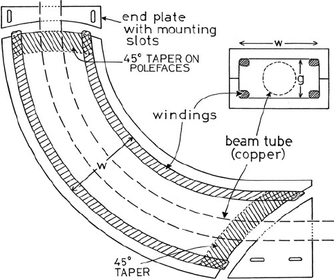
Fig. 2.9 Cross sections (in the x–z and x–y planes) through an aberration-corrected spectrometer
with curved and tapered polepiece edges, soft-magnetic mirror plates, and window-frame excita-
tion coils. The magnet operates in air, the vacuum being confined within a nonmagnetic “drift”
tube. From Egerton (1980b), copyright Elsevier

2.2 Optics of a Magnetic Prism Spectrometer 49
that must be provided in the mirror plates to allow the electron beam to enter and
leave the spectrometer (Fig. 2.9). The remaining discrepancy between the effective
and mechanical edge depends on the polepiece gap, on the separation of the field
clamps from the magnet, and on the radius of curvature of the edges (Heighway,
1975).
The effect of the fringing field on spectrometer focusing can be specified in terms
of the gap length g and a shape parameter K
1
defined by
K
1
=
∞
−∞
B
y
(z
)[B −B
y
(z
)]
gB
2
dz
(2.7)
where b
y
(z
)isthey-component of induction at y = 0 and at a perpendicular distance
z
from the polepiece edge; B is the induction between the polepieces within the
interior of the spectrometer. The SCOFF approximation corresponds to K
1
= 0; the
use of tapered polepiece edges and mirror plates, as specified above, gives K
1
≈
0.4. If the fringing field is not clamped by mirror plates, the value of K
1
is higher:
approximately 0.5 for a square-edged magnet and 0.7 for tapered polepiece edges
(Brown et al., 1977). If the polepiece gap is large, a second coefficient K
2
may be
necessary to properly describe the effect of the fringing field; however, its effect is
small for g/R < 0.3 (Heighway, 1975).
2.2.1.2 Matrix Notation
Particularly when fringing fields are taken into account, the equations needed to
describe the focusing properties of a magnetic prism become quite complicated.
Their form can be simplified and the method of calculation made more systematic
by using a matrix notation, as in the design of light-optical systems. The optical path
between object and image is divided into sections and a transfer matrix written down
for each section. The first stage of the electron trajectory corresponds to drift in a
straight line through the field-free region between the object plane and the entrance
edge of the magnet. The displacement coordinates (x, y, z) of an electron change, but
not its angular coordinates (x
= dx/dz , y
= dy/dz). Upon arrival at the entrance
edge of the magnet, these four coordinates are therefore given by the following
matrix equation:
⎛
⎜
⎜
⎝
x
x
y
y
⎞
⎟
⎟
⎠
=
⎛
⎜
⎜
⎝
1 u 00
0100
001u
0001
⎞
⎟
⎟
⎠
⎛
⎜
⎜
⎝
x
0
x
0
y
0
y
0
⎞
⎟
⎟
⎠
(2.8)
Here, x
0
and y
0
are the components of electron displacement at the object plane, x
0
and y
0
are the corresponding angular components, and the 4 × 4 square matrix is
the transfer matrix for drift over a distance u (measured along the optic axis).
The electron then encounters the focusing action of the tilted edge of the mag-
net. In the SCOFF approximation, the focusing powers are 1/f
x
=−(tan ε)/R and
50 2 Energy-Loss Instrumentation
1/f
y
= (tan ε)/R. The focusing being of equal magnitude but opposite sign in the
x- and y-directions, the magnet edge is equivalent to a quadrupole lens. Allowing
for extended fringing fields, the corresponding transfer matrix is (Brown, 1967)
⎛
⎜
⎜
⎝
10 0 0
R
−1
tan ε
1
100
00 1 0
00−R
−1
tan(ε
1
−ψ
1
)1
⎞
⎟
⎟
⎠
(2.9)
where ψ
1
represents a correction for the extended fringing field, given by
ψ
1
≈ (g/R)K
1
(1 +sin
2
ε
1
)/ cos ε
1
(2.10)
The t hird part of the trajectory involves bending of the beam within the interior of
the magnet. As discussed in Section 2.1.1, the uniform magnetic field has a positive
(convex) focusing action in the x-direction but no focusing action in the y-direction.
The effect is equivalent to that of a dipole field, as produced by a sector magnet
with ε
1
= ε
2
= 0. If φ is the bend angle, the corresponding transfer matrix can be
written i n the form (Penner, 1961)
⎛
⎜
⎜
⎝
cos φ R sin φ 00
−R
−1
sin φ cos φ 00
0010
0001
⎞
⎟
⎟
⎠
(2.11)
Upon arrival at the exit edge of the prism, the electron again encounters an effective
quadrupole, whose transfer matrix is specified by Eqs. (2.9) and (2.10) but with ε
2
substituted for ε
1
. Finally, after leaving the prism, the electron drifts to the image
plane, its transfer matrix being identical to that in Eq. (2.8) but with the object
distance u replaced by the image distance v.
Following the rules of matrix manipulation, the five transfer matrices are multi-
plied together to yield a 4 × 4 transfer matrix that relates the electron coordinates
and angles at the image plane (x
i
, y
i
, x
i
, and y
i
) to those at the object plane. However,
the first-order properties of a magnetic prism can be specified more completely by
introducing two additional parameters. One of these is the total distance or path
length l traversed by an electron, which is of interest in connection with time-of-
flight measurements but not relevant to dispersive operation of a spectrometer. The
other additional parameter is the fractional momentum deviation δ of the electron,
relative to that required for travel along the optic axis (corresponding to a kinetic
energy E
0
and zero energy loss). This last parameter is related to the energy loss
E by
δ =−E/(2γ T) (2.12)
where 2γ T = E
0
(2m
0
c
2
+E
0
)/(m
0
c
2
+E
0
). The first-order properties of the prism
are then represented by the equation

2.2 Optics of a Magnetic Prism Spectrometer 51
⎛
⎜
⎜
⎜
⎜
⎜
⎜
⎜
⎜
⎝
x
t
x
i
y
i
y
i
l
i
δ
i
⎞
⎟
⎟
⎟
⎟
⎟
⎟
⎟
⎟
⎠
=
⎛
⎜
⎜
⎜
⎜
⎜
⎜
⎜
⎜
⎝
R
11
R
12
000R
16
R
21
R
22
000R
26
00R
33
R
34
00
00R
44
R
44
00
R
51
R
52
001R
56
000001
⎞
⎟
⎟
⎟
⎟
⎟
⎟
⎟
⎟
⎠
⎛
⎜
⎜
⎜
⎜
⎜
⎜
⎜
⎜
⎜
⎝
x
0
x
0
y
0
y
0
l
0
δ
0
⎞
⎟
⎟
⎟
⎟
⎟
⎟
⎟
⎟
⎟
⎠
(2.13)
Many of the elements in this 6 ×6 matrix are zero as a result of the mirror symmetry
of the spectrometer about the x–z plane. Of the remaining coefficients, R
11
and R
33
describe the lateral image magnifications (M
x
and M
y
)inthex- and y-directions. In
general, R
11
= R
33
, so the image produced by the prism suffers from rectangular
distortion. For a real image, R
11
and R
33
are negative, denoting the fact that the
image is inverted about the optic axis. R
22
and R
44
are the angular magnifications,
approximately equal to the reciprocals of R
11
and R
33
, respectively.
Provided the spectrometer is double focusing and the value of the final drift
length used in calculating the R-matrix corresponds to the image distance, R
12
and R
34
are both zero. If the spectrometer is not double focusing, R
12
= 0atthe
x-focus and the magnitude of R
34
gives an indication of the length of the line focus
in the y-direction. To obtain good energy resolution from the spectrometer, R
12
should be zero at the energy-selection plane and R
34
should preferably be small.
The other matrix coefficient of interest in connection with energy-loss spectroscopy
is R
16
= ∂x
i
/∂(δ
0
), which relates to the energy dispersion of the spectrometer. Using
Eq. (2.12), the dispersive power D =−∂x
i
/∂E is given by
D = R
16
/(2γ T) (2.14)
The R-matrix of Eq. (2.13) can be evaluated by multiplication of the individual
transfer matrices, provided the values of u, ε
1
, φ, ε
2
, K
1
, g, and v are specified.
Such tedious arithmetic is best done by computer, for example, by running the
TRANSPORT program (Brown et al., 1977). This program
1
also computes second-
and third-order focusing, the effects of other elements (e.g., quadrupole or sextupole
lenses), of a magnetic field gradient or inhomogeneity, and of stray magnetic fields.
2.2.2 Higher Order Focusing
The matrix notation is well suited to the discussion and calculation of second-
order properties of a magnetic prism. Using the same six coordinates (x, x
, y,
y
, l, and δ), second derivatives in the form (for example) ∂
2
x
i
/∂x
0
∂x
0
can be
defined and arranged in the form of a 6 × 6 × 6 T-matrix, analogous to the first-
order R-matrix. Many of the 6
3
= 216 second-order T-coefficients are zero or
1
Available from http://www.slac.stanford.edu/pubs/slacreports/slac-r-530.html

52 2 Energy-Loss Instrumentation
are related to one another by midplane symmetry of the magnet. For energy-loss
spectroscopy, where the beam diameter at the object plane (i.e., the source size)
is small and where image distortions and off-axis astigmatism are of little signifi-
cance, the most important second-order matrix elements are T
122
= ∂
2
x
i
/∂(x
0
)
2
and
T
144
= ∂
2
x
i
/∂(y
0
)
2
. These coefficients represent second-order aperture aberrations
that increase the image width in the x-direction and therefore degrade the energy
resolution, particularly in the case of a large spread of incident angles (x
0
and y
0
).
Whereas the first-order focusing of a magnet boundary depends on its effective
quadrupole strength (equal to −tan ε =−∂z/∂x in the SCOFF approximation),
the second-order aperture aberration depends on the effective sextupole strength:
−(2ρ cos
3
ε)
−1
in the SCOFF approximation (Tang, 1982a). The aberration coeffi-
cients can therefore be varied by adjusting the angle ε and curvature ρ = ∂
2
z/∂x
2
of
the boundary. Convex boundaries can only correct second-order aberration for elec-
trons traveling in the x–y plane (T
122
= 0), but if one boundary is made concave,
the aberration for electrons traveling out of the radial plane can also be corrected
(T
122
= T
144
= 0). Alternatively, the correction can be carried out by means of
magnetic or electrostatic sextupole lenses placed before and after the spectrometer
(Parker et al., 1978).
A second-order property that is of particular importance is the angle ψ between
the dispersion plane (the plane of best chromatic focus for a point object) and the
x-axis adjacent to the image; see Fig. 2.10. This tilt angle is related to the matrix
element T
126
= ∂
2
x
i
/∂x
0
∂(δ)by
2
tan ψ =−T
126
/(R
22
R
16
) (2.15)
The condition ψ = 0 is desirable if lenses follow the spectrometer or if a parallel-
recording detector is oriented perpendicular to the exit beam. More generally,
adjustment of ψ allows control over the chromatic aberration of whole system,
external lenses included. Another second-order coefficient of some relevance is
T
166
, which does not affect the energy resolution but specifies nonlinearity of the
energy-loss axis.
The matrix method has been extended to third-order derivatives, including
the effect of extended fringing fields (Matsuda and Wollnik, 1970; Matsuo and
Matsuda, 1971; Tang, 1982a, b). Many of the 1296 third-order coefficients are zero
as a result of the midplane symmetry, and only a limited number of the remaining
ones are of interest for energy-loss spectroscopy. The coefficients ∂
3
x
i
/∂(x
0
)
3
and
∂
3
x
i
/∂x
0
∂(y
)
2
represent aperture aberrations and (like T
122
and T
144
) may have
the same or opposite signs (Scheinfein and Isaacson, 1984). Tang (1982a) pointed
out that correction of second-order aberrations by curving the entrance and exit
edges of the magnet can increase these third-order coefficients, so that the latter
limit the energy resolution for entrance angles γ above 10 mrad. The chromatic
2
If TRANSPORT is used to calculate the matrix elements, a multiplying factor of 1000 is required
on the right-hand side of Eq. (2.15) as a result of the units (x in cm, x
in mrad, and δ in %) used in
that program.
2.2 Optics of a Magnetic Prism Spectrometer 53
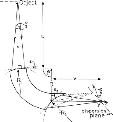
Fig. 2.10 Electron optics of
a double-focusing
spectrometer with curved
polefaces. The y-axis and the
applied magnetic field are
perpendicular to the plane of
the diagram. The
polepiece-tilt angles (ε
1
and
ε
2
) refer to the central
trajectory (the optic axis).
Exit trajectories of
energy-loss electrons are
shown by dashed lines.From
Egerton (1980b), copyright
Elsevier
term ∂
3
x
i
/∂(δ)
3
causes additional nonlinearity of the energy-loss axis but is
likely to be important only for energy losses of several kiloelectron volts. The
coefficients ∂
3
x
i
/∂(x
0
)
2
∂(δ), ∂
3
x
i
/∂(y
0
)
2
∂(δ), and ∂
3
x
i
/∂(x
0
)∂(δ)
2
introduce tilt
and curvature of the dispersion plane, which may degrade the energy resolution
when a parallel-recording system is used.
If third-order aberrations are s uccessfully corrected, for example, by the use
of octupole lenses outside the spectrometer (Tang, 1982b; Krivanek et al., 2008),
the energy resolution is limited by the fourth-order aberrations: ∂
4
x
i
/∂(x
0
)
4
,
∂
4
x
i
/∂(y
0
)
4
, and ∂
4
x
i
/∂(x
0
)
2
∂(y
0
)
2
. Fourth-order matrix theory has not been devel-
oped but ray-tracing programs can be used to predict the focusing of electrons. They
work by evaluating the rate of change of momentum as (–e)(v × B) and using this
information to define an electron path, initially the optic axis. A trajectory originat-
ing from the center of the object plane but at a small angle relative to the optic axis
is then evaluated, where this ray arrives back at the optic axis defines the Gaussian
image plane. The positions on this plane of electrons with increasing angular devia-
tion define an aberration figure (or spot diagram), from which aberration coefficients
can be estimated. One program that implements ray tracing is SIMION (http://
simion.com), which runs on Windows and Linux computers.
Spectrometer aberrations are particularly important in the case of core-loss spec-
troscopy involving higher energy ionization edges, where the angular range of the
inelastic scattering can extend to tens of milliradians and where high collection
efficiency is desirable to obtain adequate signal.
2.2.3 Spectrometer Designs
To illustrate the above concepts, we outline a procedure for designing a double-
focusing spectrometer with aperture aberrations corrected to second order by
54 2 Energy-Loss Instrumentation
curving the entrance and exit edges. First of all, the prism angles are chosen so
as to obtain suitable first-order focusing. As discussed below, the value of ε
1
should
either be fairly large (close to 45
◦
) or quite small (<10
◦
, or even negative). Knowing
the location of the spectrometer object point and the required bend radius R (which
determines the energy dispersion D and the size and weight of the magnet), approx-
imate values of ε
2
and v can be calculated using Eqs. (2.4) and (2.5). If either v or
ε
2
turns out to be inconveniently large, a different value of ε
1
must be selected.
These first-order parameters are then refined to take account of extended fringing
fields, requiring a knowledge of the integral K
1
(which depends on the shape of the
polepiece corners and on whether magnetic field clamps are to be used) and the
polepiece gap g (typically 0.1R–0.2R). The TRANSPORT program uses a fitting
procedure to find the exact image distance v corresponding to an x-focus (R
12
= 0).
The value of R
34
will then be nonzero, indicating a line focus. If
|
R
34
|
is excessive
(>1 μm/mrad), either ε
1
or ε
2
is changed slightly to obtain a closer approach to
double focusing. The dispersive power of the spectrometer is estimated from Eq.
(2.6) or obtained more accurately using Eq. (2.14).
The next stage is to determine values of the edge curvatures R
1
and R
2
that make
the second-order aperture aberrations zero. This is most easily done by recognizing
that T
122
and T
144
both vary linearly with the edge curvatures. In other words,
−T
122
= a
0
+a
1
(R/R
1
) +a
2
(R/R
2
) (2.16)
−T
144
= b
0
+b
1
(R/R
1
) +b
2
(R/R
2
) (2.17)
where a
0
, a
1
,a
2
, b
0
, b
1
, and b
2
are constants for a given first-order focusing. In
general, a
0
is positive but a
1
and a
2
are negative; T
122
can therefore be made zero
with R
1
and R
2
both positive, implying convex entrance and exit edges. However,
b
0
, b
1
, and b
2
are usually all positive so T
144
= 0 requires that either R
1
or R
2
be
negative, indicating a concave edge (Fig. 2.10). The required edge radii (R
∗
1
and R
∗
2
)
are found empirically by using the matrix program to calculate T
122
and T
144
for
three arbitrary pairs of R/R
1
and R/R
2
, such as (0, 0), (0, 1), and (1, 0), generating
six simultaneous equations that can be solved for a
0
, a
1
, a
2
, b
0
, b
1
, and b
2
. Then R
∗
1
and R
∗
2
are deduced by setting T
122
and T
144
to zero in Eqs. (2.16) and (2.17).
Not all spectrometer geometries yield reasonable values of R
∗
1
and R
∗
2
. For exam-
ple, the completely symmetric case (u = v = 2R, ε
1
= ε
2
= 26.6
◦
for φ = 90
◦
in
the SCOFF approximation) gives R
∗
1
= R
∗
2
= 0, corresponding to infinite curvature.
As
|
ε
1
−ε
2
|
increases, the necessary edge curvatures must be kept reasonably low
because the maximum effective width w
∗
of the polepieces at the entrance or exit
edge is given by
w
∗
= 2
R
∗
(1 −sin
|
ε
|
) (2.18)
for a concave edge and by w
∗
= 2R
∗
(cos ε) for a convex edge. In practice, the
concave edge corresponds to the higher value of ε,so(forsmallR
∗
)Eq.(2.18)
imposes an upper limit on the angular range (x
) of electrons that can pass through
2.2 Optics of a Magnetic Prism Spectrometer 55
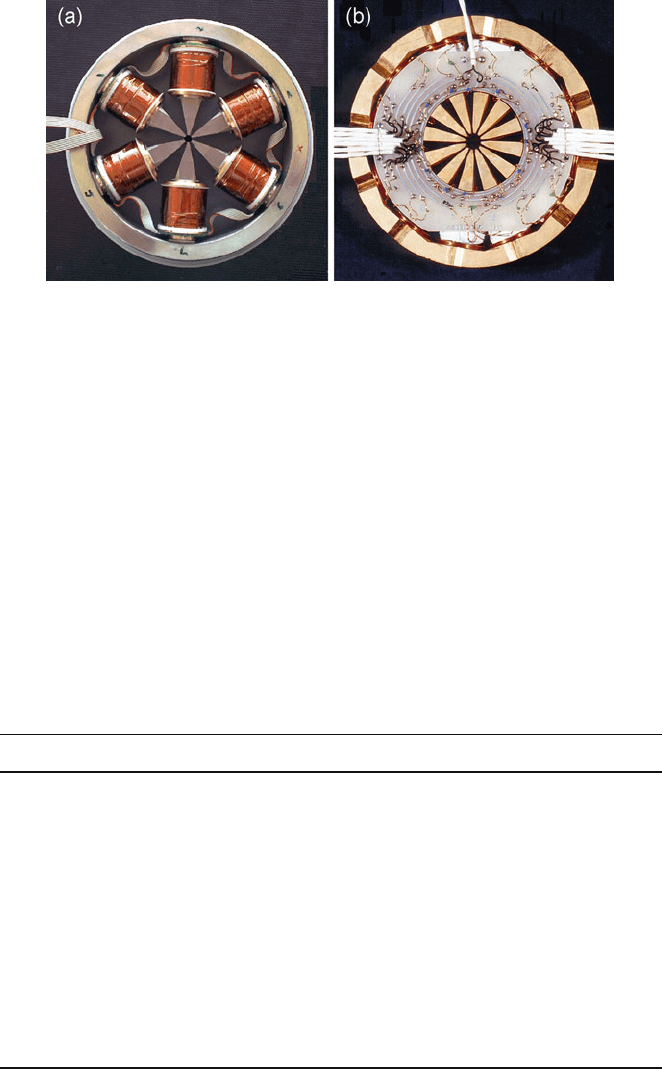
Fig. 2.11 (a) Magnetic sextupole and (b) multipole lens, used to correct the aberrations of a TEM
lens or a spectrometer. Courtesy of Max Haider, CEOS GmbH
the magnet. This limitation is not present if aberrations are adjusted by means of
external sextupoles. With the addition of external octupoles, third-order aberrations
to be corrected (Krivanek et al., 2008). Such multipole devices are also used to
correct the aberrations of axially symmetric imaging lenses; see Fig. 2.11.
In the above analysis, the object distance u and bend radius R were assumed to be
fixed by the geometry of an electron microscope column and the space available for
the spectrometer. If the ratio u/R can be varied, there is freedom to adjust a further
second-order matrix element, such as T
126
.Parkeretal.(1978) showed that there
can be two values of image (or object) distance for which T
126
= 0, giving zero tilt
of the dispersion plane.
Table 2.1 gives examples of aberration-corrected designs. The recent GIF
Quantum spectrometer (Gubbens et al., 2010) uses a gradient field design to reduce
Table 2.1 Design parameters for aberration-corrected spectrometers
φ (deg) ε
1
(deg) ε
2
(deg) u/Rv/RR
∗
1
/RR
∗
2
/Rg/R Reference
60 14.64 18.07 ∞ 1.46 1.351 −2.671 0.07 Fields (1977)
90 0 45.0 1.45 2.16 0.807 −1.357 0.2 Egerton (1980b)
70 11.75 28.79 3.60 2.38 0.707 −0.603 0.137 Shuman (1980)
90 17.5 45.0 5.5 0.98 1.0 −0.496 0.125 Krivanek and
Swann (1981)
66.6 −15 45.8 2.25 2.06 2.34 −1.30 0.18 Tang (1982a)
90 15.9 46.5 4.52 1.08 0.867 −0.500 0.19 Reichelt and Engel
(1984)
80 14.6 35.1 3.5 1.82 0.728 −0.576 0.25 Scheinfein and
Isaacson (1984)
90 16 47 6.2 0.9 1.0 −0.42 0.125 Krivanek et al.
(1995)
90 0 0 10.9 0.7 ∞∞ 0.227 Gubbens et al.
(2010)
56 2 Energy-Loss Instrumentation
the poleface angles (ε
1
and ε
2
). The pole faces are not curved; aberration correction
(including partial fourth and fifth orders) is achieved by means of three external
dodecupole (12-pole) lenses, one before the prism and two between the prism and
the energy-selecting slit. The poles of these lenses can be individually excited to
generate any combination of dipole, quadrupole, sextupole, and higher order ele-
ments, in order to control the prism focusing up to sixth order. Because these
different elements share the same optic axis, alignment is easier than with sepa-
rate elements. A further five dodecupoles (after the slit) project a spectrum or an
energy-filtered image onto the CCD detector.
2.2.4 Practical Considerations
The main aim when designing an electron spectrometer is to achieve good energy
resolution even in the presence of a large spread γ of entrance angles, enabling
the spectrometer system to have a high collection efficiency (see Section 2.3). For
γ = 10 mrad, correction of second-order aberrations allows a resolution ≈1eVfor
energy losses up to 1 keV (Krivanek and Swann, 1981; Colliex, 1982; Scheinfein
and Isaacson, 1984). The value of γ is limited by the internal diameter of the “drift”
tube (Fig. 2.9), which is necessarily less than the magnet gap g, so the historical
trend has been toward relatively large g/R ratios (see Table 2.1), even though this
makes accurate calculation of the fringing-field properties more difficult (Heighway,
1975). The use of multipole elements, giving partial correction up to fifth order, can
provide a resolution below 0.1 eV (Gubbens et al., 2010).
The energy range falling on the detector depends on the bend radius R and the
dispersion D, which increases with decreasing beam energy E
0
. In the standard (SR)
version of the GIF Quantum spectrometer, the bend radius R has been reduced from
100 to 75 mm, allowing 2 keV range for 200 keV electrons or 682 eV at 60 keV. An
even smaller value (50 mm) is scheduled for lower-voltage TEMs (15–60 keV) and
a larger one (200 mm) for high-voltage operation (400–1250 keV).
Spectrometer designs such as those in Table 2.1 assume that the magnetic induc-
tion B within the magnet is uniform or (in the gradient field case) varies linearly with
distance x from the optic axis. More generally, the induction might vary according to
B(x) = B(0)[1 − n(x/R) − m(x/R)
2
+···] (2.19)
where the coefficients n, m, ...introduce multipole components in the focusing. In
a gradient field spectrometer the value of n depends on the angle between the pole-
faces, which controls first-order focusing in the x- and y-directions, as an alternative
to tilting the entrance and exit faces. Likewise, a sextupole component (dependent
on m) could be deliberately added to control s econd-order aberrations (Crewe and
Scaduto, 1982). However, the focusing properties are quite sensitive to the values
of n and m; matrix calculations suggest that changing m by two parts in 10
−6
will
degrade the energy resolution by 1 eV, for γ = 10 mrad (Egerton, 1980b). Therefore
2.2 Optics of a Magnetic Prism Spectrometer 57
unintended variations must be avoided if a spectrometer is to behave as designed.
A“C-core” magnet (where the magnetic field is generated by a coil connected
by side arms to the polepieces) does not provide the required degree of unifor-
mity, whereas a more symmetrical arrangement with window frame coils placed
on either side of the gap (Fig. 2.9) can give a sufficiently uniform field, particularly
if the separation between the planes of the two coils is carefully adjusted (Tang,
1982a).
Further requirements for field uniformity are that the magnetic material is suffi-
ciently homogeneous and adequately thick. Homogeneity is achieved by annealing
the magnet after machining and by choosing a material with high relative perme-
ability μ and low coercivity at low field strength, such as mu-metal. Its minimum
thickness t can be estimated by requiring the magnetic reluctance (∝ w/tμ) of each
polepiece (in the x-direction) to be much less than the reluctance of the gap (∝g/w),
giving
t >> w
2
/(μg) (2.20)
Equation (2.20) precludes the use of thin magnetic sheeting, which would otherwise
be attractive in terms of reduced weight of the spectrometer.
It might appear that B-uniformity of 2×10
−16
would r equire the polepiece gap to
be uniform to within 2 μm over an x-displacement of 1 cm, for g = 1 cm. However,
the allowable variation in field strength is that averaged over the whole electron
trajectory, variations in the z-direction having less effect on the focusing. Also, pro-
vided they are small, the x- and x
2
-terms in Eq. (2.19) can be corrected by external
quadrupole and sextupole coils.
A substantial loss of energy resolution can occur if stray magnetic fields penetrate
into the spectrometer. Field penetration can be reduced by enclosing the magnet and
(more importantly) the entrance and exit drift spaces in a soft magnetic material such
as mu-metal. Such screening is usually not completely effective but the influence of
a remaining alternating field can be canceled by injecting a small alternating current
into the spectrometer scan coils, as described in Section 2.2.5.
The magnetic induction within the spectrometer is quite low (<0.01 T for
100 keV operation) and can be provided by window frame coils of about 100 turns
carrying a current of the order of 1 A. To prevent drift of the spectrum due to changes
in temperature and resistance of the windings, the power supply must be current
stabilized to within one part in 10
6
for 0.3-eV stability at 100-keV incident energy.
Stability is improved if the power supply is left running continuously.
2.2.5 Spectrometer Alignment
Like all electron-optical elements, the magnetic prism performs t o its design spec-
ifications only if it is correctly aligned relative to the incoming beam of electrons.
Since the energy dispersion is small for high-energy electrons, this alignment is
fairly critical if the optimum energy resolution is to be achieved.