Enns R.H. Computer Algebra Recipes for Mathematical Physics

Подождите немного. Документ загружается.

9.1. ORDINARY DIFFERENTIAL EQUATIONS 349

Consider the following pair of coupled ﬁrst-order linear ODEs with time-

dependent forcing terms present in each equation,

˙x =9x +24y +5cost −

sin t, ˙y = −24 x − 51 y − 9cost +

sin t.

Suppose that the initial condition is x(0) = 4/3, y(0) = 2/3. Let’s begin the

recipe by entering the ODE system and the initial condition.

restart: with(plots):

sys:=diff(x(t),t)=9*x(t)+24*y(t)+5*cos(t)-(1/3)*sin(t),

diff(y(t),t)=-24*x(t)-51*y(t)-9*cos(t)+(1/3)*sin(t);

sys :=

x(t)=9x(t)+24y(t) + 5 cos(t) −

sin(t),

y(t)=−24 x (t) − 51 y(t) − 9 cos(t)+

sin(t)

ic:=x(0)=4/3,y(0)=2/3:

The analytic forms of x(t)andy(t) follow on applying the dsolve command to

sys, subject to the initial condition.

sol:=dsolve({sys,ic},{x(t),y(t)});

sol := {x (t)=−e

(−39 t)

+2e

(−3 t)

cos(t), y(t)=2e

(−39 t)

−e

(−3 t)

−

cos(t)}

There are two widely diﬀering characteristic times in the transient part of the

solution, viz., τ

=1/39  0.03 and τ

=1/3  0.3. The shorter time τ

will

set an approximate boundary between the stability or the lack thereof of the

RK4 scheme. For later comparison, let’s plot the exact solution, ﬁrst using the

following operator F to select the forms of x and y separately from sol.

F:=v->rhs(select(has,sol,v(t))[1]):

Then, using F with v =x and y, the exact analytic solution is plotted, using the

spacecurve command, in the 3-dimensional t vs. x vs. y space.

gr:=spacecurve([t,F(x),F(y)],t=0..20,numpoints=2000):

An operator sol2 is formed to numerically solve the ODE system, for a speciﬁed

stepsize h, using the fourth-order RK algorithm.

sol2:=h->dsolve({sys,ic},{x(t),y(t)},numeric,stepsize=h,

method=classical[rk4]):

An operator G is created to plot the numerical solution s for a speciﬁed h and

upper time limit T. The latter is included because for h>>τ

, but less than

, numerical overﬂow will occur if we try to plot the RK4 solution for large T .

G:=(s,h,T)->odeplot(s(h),[t,x(t),y(t)],t=0..T,numpoints=2000,

style=line,axes=box,labels=["t","x","y"]):

Using G, the RK4 numerical solution is plotted for h =0.05 and T =20 and

superimposed on the exact solution (plotted in gr)withthedisplay command.

display({gr,G(sol2,0.05,20)});

350 CHAPTER 9. NUMERICAL METHODS

–1

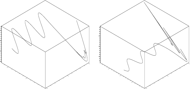
Figure 9.5: Left: Exact & RK4 curves (h=.05). Right: RK4 & RKF45 (h=.08).

The resulting picture is shown on the left of Figure 9.5, the exact solution being

the completely smooth curve, the RK4 numerical solution deviating away from

the exact result during the transient interval but locking onto the steady-state

oscillatory solution for larger times. The slight deviation of the RK4 solution

away from the exact curve is a precursor of the onset of numerical instability

which occurs if h is increased much further. Before showing what happens, let’s

form another operator sol3 to numerically solve the ODE system for a given h

using the RKF 45 algorithm.

sol3:=h->dsolve({sys,ic},{x(t),y(t)},numeric,method=rkf45):

Now the time stepsize h is increased to 0.08, which is still substantially less

than the other characteristic time τ

 0.3 in the problem. The RK4 and RKF

45 solutions for h =0.08 are now superimposed with the display command,

the resulting curves being shown on the right of Figure 9.5.

display({G(sol2,0.08,0.21),G(sol3,0.08,20)});

The jagged diverging curve is the RK4 solution, the smooth one the RKF 45

result. For the RKF 45 solution, derived with sol3, the upper time limit is

still 20, but for the RK4 solution, derived with sol2, T has been shortened to

0.21 to avoid ﬂoating point overﬂow. Noting that the x and y scales of the two

viewing boxes in Figure 9.5 are diﬀerent, the RKF 45 result agrees with the

analytical result.

It should be mentioned that other numerical algorithm options are available

for solving stiﬀ ODE systems. The reader should consult Maple’s Help under

the topic heading “dsolve,numeric” for information about these options.

9.1. ORDINARY DIFFERENTIAL EQUATIONS 351

9.1.6 A Strange Attractor

Wickedness is a myth invented by good people to account for the

curious attractiveness of others.

Oscar Wilde, Anglo-Irish playwright, author, (1854–1900)

Implicit numerical algorithms, based on replacing the exact ﬁrst derivative with

the BWDA, are stable for any ﬁxed stepsize h, although they may not be too ac-

curate if h is made too large. For nonlinear ODEs, the implicit schemes involve

solving simultaneous nonlinear algebraic equations at each step. In practice,

the algorithms are often made semi-implicit by linearizing the algebraic equa-

tions. In this recipe, a semi-implicit scheme is developed for the R¨ossler system

[Ros76], which is famous for its “top-hat” strange attractor.

The R¨ossler equations are

˙x = −(y + z) ≡ X, ˙y = x + ay ≡ Y, ˙z = b + z (x −c) ≡ Z, (9.10)

with x, y,andz real and a, b, c real, positive, constants. They were introduced

by R¨ossler to illustrate how a simple 3-dimensional ODE system can exhibit

periodic and chaotic solutions, depending on the parameter values.

Using the BWDA in the Euler method, with k replaced by k+1, (9.10) yields

k+1

= x

+ hX

k+1

= y

+ hY

k+1

= z

+ hZ

k+1

. (9.11)

This resembles the Euler algorithm that was used before, except now the rhs

of (9.10) are evaluated at the “new” time step instead of the “old” one. This

is an example of an implicit scheme. If all the ODEs are linear, it is easy to

solve the equations, expressing x

k+1

, y

k+1

,andz

k+1

completely in terms of

the old known values. For the R¨ossler system, Z

k+1

contains the nonlinear

term, z

k+1

, involving the new unknown values. It is customary to con-

vert implicit schemes to semi-implicit ones by Taylor expanding the nonlinear

terms around the old values. For example, for the nonlinear term in Z,wewrite

f ≡ z

k+1

= f(x

)+(x

k+1

− x

)



∂f

∂x



+(z

k+1

− z

)



∂f

∂z



+···

= x

+(x

k+1

− x

) z

+(z

k+1

− z

) x

+ ···.

Substituting this expansion into (9.11) and collecting terms yields

k+1

+ hy

k+1

+ hz

k+1

= x

−hx

k+1

+(1− ha) y

k+1

= y

−hz

k+1

+(1+hc− hx

) z

k+1

= hb+(1−hx

) z

(9.12)

This system of three linear algebraic equations is then solved on each time step.

The semi-implicit scheme derived above is only of O(h) accuracy. To derive

a second-order accurate implicit scheme, we can average

the old and the new

This is the basis of the Crank–Nicolson scheme for solving nonlinear PDEs.

352 CHAPTER 9. NUMERICAL METHODS

on the rhs, i.e., replace equations (9.11) with

k+1

),y

k+1

),z

k+1

(9.13)

Using the same expansion for the nonlinear term, a second-order semi-implicit

algorithm for solving the R¨ossler equations then is

k+1

= x

−

h (y

+ z

−

k+1

+(1−

ha) y

k+1

+(1+

ha) y

−

k+1

+(1+

hc−

) z

k+1

= hb+(1−

hc) z

(9.14)

In this recipe, we will iterate equations (9.14), taking 10 digits,

restart: with(plots): Digits:=10:

with a=b=0.2, c=5.0, h=0.05 and n=3000 iterations.

a:=0.2: b:=0.2: c:=5.0: h:=0.05: n:=3000:

The initial condition at t

=0 is x

=−1, y

=0, z

=0.

t[0]:=0: x[0]:=-1: y[0]:=0: z[0]:=0:

After recording the start time, a do loop is created to iterate eqs. (9.14)

begin:=time():

forkfrom0tondo

The rhs of each equation is entered in A1[k], A2[k],andA3[k].

A1[k]:=x[k]-0.5*h*(y[k]+z[k]);

A2[k]:=0.5*h*x[k]+(1+0.5*h*a)*y[k];

A3[k]:=h*b+(1-0.5*h*c)*z[k];

The three equations of (9.14) are entered in E1, E2,andE3.

E1:=x[k+1]+0.5*h*y[k+1]+0.5*h*z[k+1]=A1[k];

E2:=-0.5*h*x[k+1]+(1-0.5*h*a)*y[k+1]=A2[k];

E3:=-0.5*h*z[k]*x[k+1]+(1+0.5*h*c-0.5*h*x[k])*z[k+1]=A3[k];

The three algebraic equations, E1, E2, E3 are numerically solved for x

k+1

, y

k+1

and z

k+1

and the solution then assigned.

sol[k+1]:=(fsolve({E1,E2,E3},{x[k+1],y[k+1],z[k+1]}));

assign(sol[k+1]);

Thevaluesofx

k+1

, y

k+1

, z

k+1

,andt

k+1

+ h, are recorded,

x[k+1],y[k+1],z[k+1]; t[k+1]:=t[k]+h;

and the plotting point (x

, y

, z

) formed for the kth time step.

pt[k]:=[x[k],y[k],z[k]];

end do:

On ending the do loop, the cpu time for the loop is calculated

cpu:=time()-begin;

9.2. PARTIAL DIFFERENTIAL EQUATIONS 353

cpu := 10.242

and found to be about 10 seconds. Using the spacecurve command with a line

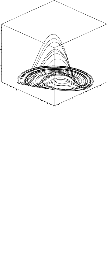
style and zhue coloring, the solution is plotted and shown in Figure 9.6.

spacecurve([seq(pt[j],j=0..n)],style=line,shading=zhue,

orientation=[45,60],axes=boxed,labels=["x","y","z"]);

–5

Figure 9.6: R¨ossler’s strange attractor.

After an initial transient period, the trajectory is attracted to a localized region,

where it continually traces out a new path, i.e., the motion is chaotic. This

localized chaotic motion, resembling a man’s “top hat”, is an example of what

mathematicians call a strange attractor. Starting with some other initial values

of x

, y

,andz

, you will ﬁnd that the trajectory is eventually attracted to

the top hat region. For other values of the parameters, periodic motions can

also be observed. As an exercise, try varying the parameter c, holding all other

parameter values ﬁxed.

9.2 Partial Diﬀerential Equations

Finite diﬀerence approximations can also be used to numerically solve PDEs.

For example, our ﬁrst recipe involves ﬁnding the steady-state temperature

T (x, y) inside a thin rectangular plate with speciﬁed temperatures on the four

edges. T (x, y) will satisfy the 2-dimensional form of Laplace’s equation,

∂

∂x

∂

∂y

=0. (9.15)

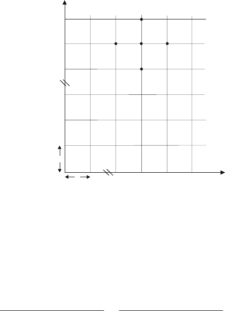
Our approach is to divide the x-y plane into a rectangular grid or “mesh”, as

shown in Figure 9.7, with each small rectangle having sides of length h and k.

354 CHAPTER 9. NUMERICAL METHODS

0,0 1,0

0,1 1,1

0,2 1,2

i-1,ji, ji+1, j

i, j-1

i, j+1

y = jk

x = ih

Figure 9.7: Subdividing the x-y plane with a numerical mesh.

The coordinates of a typical mesh (intersection) point P are x = ih, y = jk,

with i, j =0, 1, 2, .... The mesh points may be labeled by a pair of integers,

the point P being indicated by (i, j), and the temperature at that point by

i,j

≡ T (x = ih,y= jk). From Chapter 2, each second derivative in Laplace’s

equation can be replaced with a central diﬀerence approximation (CDA), viz.,

i+1,j

− 2 T

i,j

+ T

i−1,j

)

i,j+1

− 2 T

i,j

+ T

i,j−1

)

=0, (9.16)

or, on setting r =(h/k)

and rearranging,

2(1+r) T

i,j

− T

i+1,j

− T

i−1,j

− rT

i,j+1

− rT

i,j−1

=0. (9.17)

For a given point P , the mesh points involved in (9.17) are as shown in Fig-

ure 9.7. If the temperature is speciﬁed at the mesh points making up the

boundary of the plate, equation (9.17) can be used to calculate the tempera-

ture at each of the internal mesh points, as will now be demonstrated.

9.2.1 Steady-State Temperature Distribution

If you can’t stand the heat, get out of the kitchen.

Harry S. Truman, former American president, (1884–1972)

A thin rectangular plate, with 0 ≤ x ≤ L1=1/2and0≤ y ≤ L2 = 1, has the

following temperature distributions along its four edges: T(x, 0) =500 x (L1−x),

T (x, L2) = 700 x (L1 − x), T (0,y)=0, T (L1,y) = 1000 y (L2 − y). Dividing the

plate into a numerical mesh with 15 steps in the x direction and 30 steps in the

y direction, determine and plot the temperature proﬁle inside the plate.

9.2. PARTIAL DIFFERENTIAL EQUATIONS 355

The plots library package is loaded and the start time recorded.

restart: with(plots): begin:=time():

The values L1=1/2, L2 = 1, and the numbers of steps, m =15 and n = 30, are

entered. The corresponding stepsizes h = L1/m and k = L2/n are calculated,

along with the ratio r =(h/k)

L1:=1/2: L2:=1: m:=15: n:=30: h:=L1/m; k:=L2/n; r:=(h/k)ˆ2;

h :=

k :=

r := 1

The x and y coordinates of the mesh points are generated.

Xcoords:=seq(x[i]=i*h,i=0..m): Ycoords:=seq(y[j]=j*k,j=0..n):

The temperature distributions along the four edges are evaluated at the bound-

ary mesh points by setting x= ih and y = jk.

bc1:=seq(T[i,0]=500*i*h*(L1-i*h),i=0..m):

bc2:=seq(T[i,n]=700*i*h*(L1-i*h),i=0..m):

bc3:=seq(T[0,j]=0,j=0..n):

bc4:=seq(T[m,j]=1000*j*k*(L2-j*k),j=0..n):

The x and y mesh point coordinates and the 4 boundary conditions are assigned.

assign(Xcoords,Ycoords,bc1,bc2,bc3,bc4):

A functional operator f is formed to calculate the lhs of equation (9.17).

f:=(i,j)->2*(1+r)*T[i,j]-T[i+1,j]-T[i-1,j]-r*T[i,j+1]

-r*T[i,j-1];

f := (i, j) → 2(1+r) T

i, j

− T

i+1,j

− T

i−1,j

− rT

i, j+1

− rT

i, j−1

Making use of f and a nested sequence command, the equations which have to

be solved at the (m − 1) × (n −1) internal mesh points are generated.

eqs:={seq(seq(f(i,j)=0,i=1..m-1),j=1..n-1)}:

The (m − 1) ×(n −1) unknown temperature variables T

i,j

are entered.

vars:={seq(seq(T[i,j],i=1..m-1),j=1..n-1)}:

The mesh equations are then numerically solved for the variables, the answers

being given to 6 digits. The solution is then assigned.

sol:=evalf(fsolve(eqs,vars),6): assign(sol):

We now create the plotting points (x

, y

, T

i,j

)fori=0 to m and j =0 to n.

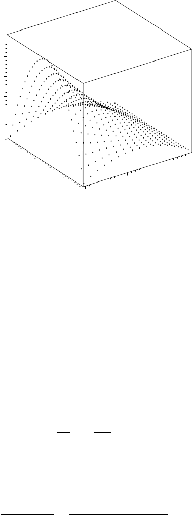
pts:=seq(seq([x[i],y[j],T[i,j]],i=0..m),j=0..n):

The numerical points are plotted with the pointplot3d command, being rep-

resented by size 6 circles which are colored with the zhue shading option. The

resulting temperature proﬁle inside the 3-dimensional viewing box is as shown

in Figure 9.8. The box can be rotated in the usual manner.

pointplot3d([pts],symbol=circle,symbolsize=6,shading=zhue,

axes=boxed,orientation=[55,60],labels=["x","y","T"]);

356 CHAPTER 9. NUMERICAL METHODS

0.5

250

Figure 9.8: Numerically obtained temperature proﬁle inside plate.

The cpu time for the entire recipe is about 13 seconds.

cpu:=time()-begin;

cpu := 13.361

9.2.2 1-Dimensional Heat Flow

In general, the art of government consists in taking as much money

as possible from one party of the citizens to give to the other.

Francois Voltaire, French philosopher, (1696–1778)

One-dimensional heat ﬂow is governed by the temperature diﬀusion equation

∂T

∂t

= σ

∂

∂x

, (9.18)

with x the spatial coordinate, t the time, and σ the heat diﬀusion coeﬃcient.

Setting y = σt, a numerical algorithm can be formed by replacing the second

order x derivative with a CDA (spatial step, h)andtheﬁrstordery derivative

by a FWDA (y step, k), viz.,

i,j+1

− T

i,j

i+1,j

− 2 T

i,j

+ T

i−1,j

, (9.19)

or, on setting r = k/h

and rearranging,

i,j+1

= rT

i−1,j

+(1− 2 r) T

i,j

+ rT

i+1,j

. (9.20)

9.2. PARTIAL DIFFERENTIAL EQUATIONS 357

In terms of a “mesh diagram” for the x-y plane, the mesh points involved in

(9.20) are as shown in Figure 9.9. The unknown temperature T

i,j+1

is to be

explicitly determined on the j + 1st time step from the three known values

i−1,j

, T

i,j

,andT

i+1,j

on the previous jth step.

y = j k

x = i h

T (x,0) specified

T( 0,y) = 0

, 0

T T T

i−1, j i, j i+1, j

i, j+ 1

T (L, y ) = 0

Figure 9.9: Numerical mesh for the heat ﬂow recipe.

One starts with the bottom row (j = 0) which corresponds to the speciﬁed initial

temperature distribution inside, say, a thin rod of length L, and calculates T

at each internal mesh point of the ﬁrst (j = 1) time row. With T

i,1

all known,

one proceeds to calculate T on the second time row, and so on. To implement

the algorithm, we must also specify the boundary conditions at the ends of the

rod. For example, we might have T (0,y)=T (L, y)= 0 as in the ﬁgure.

Suppose that T (x, 0) = 200 x

(L − x)withL = 1 m. To implement the

algorithm, the LinearAlgebra package is loaded so a matrix multiplication can

be used for calculating T at the internal mesh points. Let’s subdivide the range

x=0 to x= L by taking N = 25 internal grid points. The relevant matrix A for

implementing the rhs of (9.20) will be an N ×N tridiagonal matrix, with 1 −2 r

along the main diagonal, r along the ﬁrst subdiagonals, and zeros everywhere

else. For N>10, the matrix will not be explicitly displayed unless rtablesize

is set to N or larger in the interface command. Here it is set to inﬁnity.

restart: with(LinearAlgebra): interface(rtablesize=infinity):

Entering N and L, the spatial stepsize is h =L/(N +1) which is now evaluated.

The explicit scheme becomes numerically unstable if r = k/h

> 1/2, so let’s

take r =0.05. Then the y stepsize k = rh

is calculated. The number of plots

to be produced in the iteration is given by numplots.

358 CHAPTER 9. NUMERICAL METHODS

N:=25: L:=1.0: h:=L/(N+1); r:=0.05: k:=r*hˆ2; numplots:=100:

h := 0.03846153846 k := 0.00007396449705

Using the BandMatrix command, the relevant matrix A is entered. The diagonal

entries are given by 1 − 2 r =0.90, the subdiagonal entries by r =0.05. The

number 1 indicates that there is one subdiagonal and N gives the size of the

matrix, i.e., N × N. For brevity, the output shown here in the text has been

truncated, only 5 of the 25 rows being shown.

A:=BandMatrix([r,1-2*r,r],1,N);

A:= [0.90, 0.05, 0, 0, 0, 0, 0, 0, 0, 0, 0, 0, 0, 0, 0, 0, 0, 0, 0, 0, 0, 0, 0, 0, 0]

[0.05, 0.90, 0.05, 0, 0, 0, 0, 0, 0, 0, 0, 0, 0, 0, 0, 0, 0, 0, 0, 0,

0, 0, 0, 0, 0]

[0, 0.05, 0.90, 0.05, 0, 0, 0, 0, 0, 0, 0, 0, 0, 0, 0, 0, 0, 0, 0, 0, 0, 0, 0, 0, 0]

[...............................................................................................................]

[0, 0, 0, 0, 0, 0, 0, 0, 0, 0, 0, 0, 0, 0, 0, 0, 0,

0, 0, 0, 0, 0, 0.05, 0.90, 0.05]

[0, 0, 0, 0, 0, 0, 0, 0, 0, 0, 0, 0, 0, 0, 0, 0, 0, 0, 0, 0, 0, 0, 0, 0.05, 0.90]

A functional operator f is formed for generating the values of the initial tem-

perature proﬁle at the internal spatial grid points.

f:=x->evalf(200*xˆ3*(L-x)):

Using f, the values of the temperature at the internal x mesh points on the

zeroth time row are formed into a column vector v. Again, only a few of the 25

entries are shown here in the text.

v:=Vector([[seq(f(i*h),i=1..N)]]);

v :=

⎡

⎢

⎣

0.01094149364

0.08403067118

0.2717867022

..................

21.01335738

..................

12.10041666

6.838433534

⎤

⎥

⎦

To establish the vertical scale of our plot, the following max command is used

to select the largest temperature value from the sequence of entries in v.

vmax:=max(seq(v[i],i=1..N));

vmax := 21.01335738

The start time for the following do loop, which carries out the requisite matrix

multiplication, is recorded.

begin:=time():

The do loop runs from n =1 to numplots. The matrix multiplication is carried

out in T, a plot being produced on every 20th time step. For plotting purposes