Francoise J.-P., Naber G.L., Tsun T.S. (editors) Encyclopedia of Mathematical Physics

Подождите немного. Документ загружается.

where i, j = 1, ..., ‘. Let

E ¼

10



denote the 2‘  2‘ matrix formed by four ‘  ‘

blocks, equal to the 0 matrix or, as indicated, to the

(identity matrix); then, if a superscript T denotes

matrix trans position, the condition that the map be

canonical is that

1

¼ EL

or L

1

B

C



½16

which immediately implies that det L = 1. In fact,

it is possible to show that [16] implies det L = 1.

Equation [16] is equivalent to the four relations AD



= 1, AB

þ BA

= 0, CD

 DC

= 0, and

CB

þ DA

= 1. More explicitly, since the first and

the fourth relations coincide, these can be expressed as

f

;

g¼

; f

;

g¼0; f

;

g¼0 ½17

where, for any two functions F(p, k), G(p, k), the

Poisson bracket is

fF; Ggðp; kÞ¼

def

‘

k¼1



Fðp; kÞ@



Gðp; kÞ



@



Fðp; kÞ@



Gðp; kÞ



½18

The latter satisfies Jacobi’s identity:{{F, G}, Q} þ

{{G, Q}, F} þ {{Q, F}, G} = 0, for any three functions

F, G, Q on the phase space. It is quite useful to

remark that if t !(p(t), q(t)) = S

(p, q) is a solution

to Hamilton equations with Hamiltonian H then,

given any observable F(p, q), it ‘‘evolves’’ as

F(t) =

def

F(p(t), q(t)) satisfying

FðpðtÞ; qðtÞÞ= {H; F}ðpðtÞ; qðtÞÞ

Requiring the latter identity to hold for all observables

F is equivalent to requiring that the t !(p(t), q(t)) be a

solution of Hamilton’s equations for H.

Let C: U ! U

be a smooth, smoothly invertible

transformation between two open 2‘-dimensional

sets: C(p, k) = (p

, k

). Suppose that there is a function

(p

, k) defined on a suitable domain W such that

Cðp; kÞ¼ðp

; k

Þ)

p ¼ @

ðp

; kÞ

¼ @

ðp

; kÞ



½19

then C is canonical. This is because [19] implies that

if k, p

are varied and if p, k

, p

, k are related by

C(p, k) = (p

, k

), then p  dk þ k

 dp

= d( p

, k),

which implies that

p  dk Hðp; kÞdt  p

 dk

 HðC

1

ðp

; k

ÞÞdt

þ dðp

; kÞdðp

 k

Þ½20

It means that the Hamiltonians H(p, q)and

, q

)) =

def

H(C

1

, q

)) have Hamilton actions

and A

differing by a constant, if evaluated

on corresponding motions (p(t), q(t)) and

(t), q

(t)) = C(p(t), q(t)).

The constant depends only on the initial and final

values (p(t

), q(t

)) and (p(t

), q(t

)) and, respec-

tively, (p

), q

)) and (p

), q

)) so that if

(p(t), q(t)) makes A

extreme, then (p

(t), q

(t)) =

C(p( t), q(t)) also makes A

extreme.

Hence, if t !(p(t), q(t)) solves the Hamilton equa-

tions with Hamiltonian H(p, q) then the motion

t !(p

(t), q

(t)) = C(p( t), q(t)) solves the Hamilton

equations with Hamiltonian H

, q

) = H(C

1

, q

))

no matter which it is: therefore, the transformation is

canonical. The function  is called its generating

function.

Equation [19] provides a way to construct

canonical maps. Suppose that a function (p

, k)is

given and defined on some domain W; then setting

p ¼ @

ðp

; kÞ

¼ @

ðp

; kÞ



and inverting the first equation in the form

= X(p, k) and substituting the value for p

thus

obtained, in the second equation, a map

C(p, k) = (p

, k

) is defined on some domain (where

the mentioned operations can be performed) and if

such domain is open and not empty then C is a

canonical map.

For similar reasons, if (k, k

) is a function

defined on some domain then setting p = @



(k, k

), p

= @

(k, k

) and solving the first rela-

tion to express k

= D(p, k) and substituting in the

second relation a map (p

, k

) = C(p, k) is defined on

some domain (where the mentioned operations can

be performed) and if such domain is open and not

empty then C is a canonical map.

Likewise, canonical transformations can be con-

structed starting from a priori given functions

F(p, k

)orG(p, p

). And the most general canonical

map can be generated locall y (i.e., near a given point

in phase space) by a single one of the above four

ways, possibly composed with a few ‘‘trivial’’

canonical maps in which one pair of coordinates

(

, 

) is transformed into (

, 

). The necessity of

also including the trivial maps can be traced to the

existence of homogeneous canonical maps, that is,

maps such that p  dk = p

 dk

(e.g., the identity

map, see below or [49] for nontrivial examples)

which are action preserving hence canonical, but

which evidently cannot be generated by a function

(k, k

) although they can be generated by a

function depending on p

, k.

Introductory Article: Classical Mechanics 5

Simple examples of homogeneous canonical maps

are maps in which the coordinates q are changed

into q

= R(q) and, correspondingly, the p’s are

transformed as p

= (@

R(q))

1T

p, linearly: indeed,

this map is generated by the function F(p

, q) =

def

 R(q).

For instance, consider the map ‘‘Cartesian–polar’’

coordinates (q

, q

) ! (, ) with (, ) the polar

coordinates of q (namely  =

ﬃﬃﬃﬃﬃﬃﬃﬃﬃﬃﬃﬃﬃﬃﬃﬃ

þ q

,  = arctan

)) and let n=

def

q=jqj=(n

) and t =(n

, n

Setting p



def

p n, p



def

p t, the map (p

, p

, q

) ! (p



, p



, , ) is homogeneous canonical

(because p dq=p nd þp td=p



d þp



d).

As a further example, any area-preserving map

(p, q) ! (p

, q

) defined on an open region of the

plane R

is canonical: because in this case the

matrices A, B, C, D are just numbers, which satisfy

AD  BC = 1 and, therefore, [16] holds.

For more details, the reader is referred to Landau

and Lifshitz (1976) and Gallavotti (1983) .

Quadratures

The simplest mechanical systems are integrable by

quadratures. For instance, the Hamiltonian on R

Hðp; qÞ¼

þ VðqÞ½21

generates a motion t !q(t) with initial data q

such that H(p

, q

) = E, i.e.,

þ V(q

) = E,

satisfying

qðtÞ¼

ﬃﬃﬃﬃﬃﬃﬃﬃﬃﬃﬃﬃﬃﬃﬃﬃﬃﬃﬃﬃﬃﬃﬃﬃﬃﬃﬃﬃﬃﬃﬃﬃﬃﬃ

ðE  VðqðtÞÞÞ

If the equation E = V(q) has only two solutions



(E) < q

(E) and j@

V(q



(E))j > 0, the motion is

periodic with period

TðEÞ¼2

ðEÞ



ðEÞ

ﬃﬃﬃﬃﬃﬃﬃﬃﬃﬃﬃﬃﬃﬃﬃﬃﬃﬃﬃﬃﬃﬃﬃﬃﬃﬃﬃﬃﬃﬃﬃﬃﬃﬃﬃﬃ

ð2=mÞðE  VðxÞÞ

½22

The special solution with initial data q



(E),

= 0 will be denoted Q(t), and it is an

analytic function (by the general regularity theorem

on ordinary differential equations). For 0  t  T=2

or for T=2  t  T it is given, respe ctively, by

t ¼

QðtÞ



ðEÞ

ﬃﬃﬃﬃﬃﬃﬃﬃﬃﬃﬃﬃﬃﬃﬃﬃﬃﬃﬃﬃﬃﬃﬃﬃﬃﬃﬃﬃﬃﬃﬃﬃﬃﬃﬃﬃ

ð2=mÞðE  VðxÞÞ

½23a

t ¼



QðtÞ

ðEÞ

ﬃﬃﬃﬃﬃﬃﬃﬃﬃﬃﬃﬃﬃﬃﬃﬃﬃﬃﬃﬃﬃﬃﬃﬃﬃﬃﬃﬃﬃﬃﬃﬃﬃﬃﬃﬃ

ð2=mÞðE  VðxÞÞ

½23b

The most general solution with energy E has the

form q(t) = Q(t

þ t), where t

is defined by

= Q(t

Q(t

), i.e., it is the time needed for

the ‘‘standard solution’’ Q(t) to reach the initial data

for the new motion.

If the derivative of V vanishes in one of the

extremes or if at least one of the two solutions q



(E)

does not exist, the motion is not perio dic and it may

be unbounded: nevertheless, it is still expressible via

integrals of the type [22]. If the potential V is

periodic in q and the variable q is considered to be

varying on a circle then essentially all solutions are

periodic: exceptions can occur if the energy E has a

value such that V(q) = E admits a solution where V

has zero derivative.

Typical examples are the harmonic oscillator, the

pendulum, and the Kepler oscillator: whose Hamil-

tonians, if m, !, g, h, G, k are positive constants, are,

respectively,

þ mg 1  cos



 mk

jqj

þ m

½24

the Kepler oscillator Hamiltonian has a potential

which is singular at q = 0 but if G 6¼ 0 the energy

conservation forbid s too close an approach to q = 0

and the singularity becomes irrelevant.

The integral in [23] is called a quadrature and the

systems in [21] are therefore integrable by quad-

ratures. Such systems, at least when the motion is

periodic, are best described in new coordinates in

which periodicity is more manifest. Namely when

V(q) = E has only two roots q



(E)andV



(E)) > 0

the energy–time coordinates can be used by replac-

ing q,

q or p, q by E, , where  is the time needed

for the standard solution t !Q(t)toreachthegiven

data, that is, Q() = q,

Q() =

q. In such coordi-

nates, the motion is simply (E, ) !(E,  þ t) and,

of course, the variable  has to be regarded as

varying on a circle of radius T=2. The E, 

variables are a kind of polar coordinates, as can

be checked by drawing the curves of constant E,

‘‘energy levels,’’ in the plane p, q in the cases in

[24]; see Figure 1.

In the harmonic oscillator case, all trajectories are

periodic. In the pendulum case, all motions are

periodic except the ones which separate the oscilla-

tory motions (the closed curves in the second

drawing) from the rotatory motions (the apparently

open curves) which, in fact, are on clos ed curves as

well if the q coordinate, that is, the vertical

6 Introductory Article: Classical Mechanics

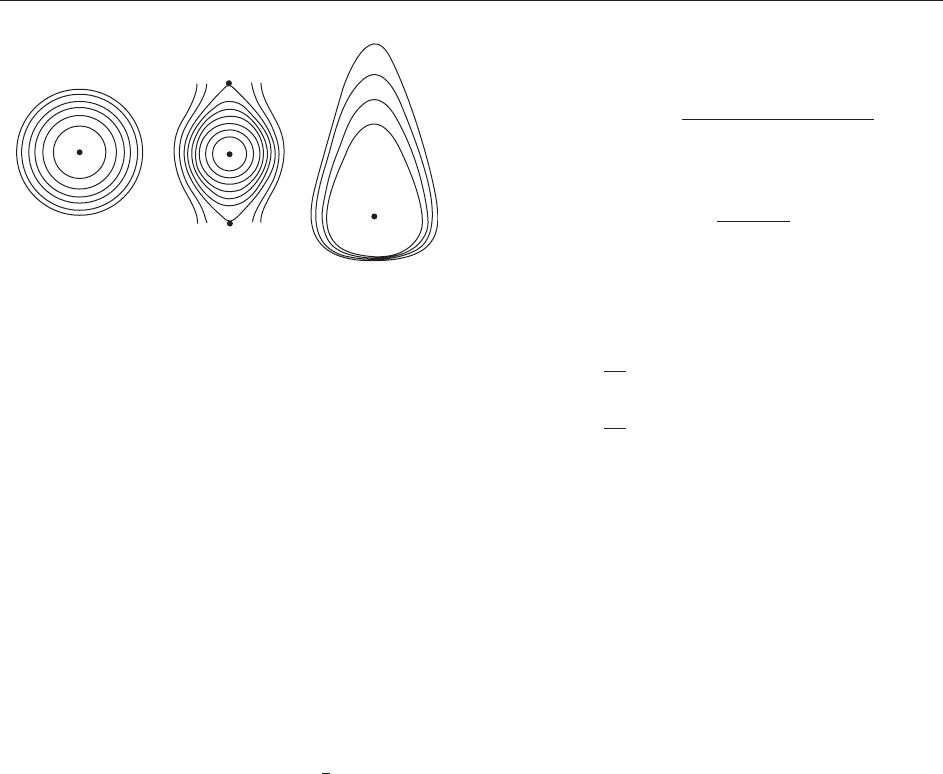
coordinate in Figure 1, is regarded as ‘‘periodic’’

with period 2h. In the Kepler case, only the

negative-energy trajectories are periodic and a few

of them are drawn in Figure 1. The single dots

represent the equilibrium points in phase space.

The r egion of phase space where motions are

periodic i s a set of points (p, q)withthe

topological structure of [

u2U

({u}  C

), where u is

a coordinate varying in a n open interval U (e.g.,

the set of values of the e nergy), and C

is a closed

curve whose points (p, q) are id entifi ed by a

coordinate (e.g., by the time necessary for an

arbitrarily fixed datum with the same energy to

evolve into (p, q)).

In the above cases, [24], if the ‘‘radial’’ coordinate

is chosen to be the energy the set U is the interval

(0, þ1) for the harmonic oscillator, (0, 2mg)or

(2mg, þ1) for the pendulum, and (

,0)in

the Kepler case. The fixed datum for the reference

motion can be taken, in all cases, to be of the form

(0, q

) with the time coordinate t

given by [23].

It is remarkable that the energy–time coordinates

are canonical coordinates: for instance, in the vicinity

of (p

, q

)andifp

> 0, this can be seen by setting

Sðq; EÞ¼

ﬃﬃﬃﬃﬃﬃﬃﬃﬃﬃﬃﬃﬃﬃﬃﬃﬃﬃﬃﬃﬃﬃﬃﬃﬃﬃﬃﬃﬃﬃ

2mðE  VðxÞÞ

dx ½25

and checking that p = @

S(q, E), t = @

S(q, E) are

identities if (p, q) and (E, t) are coordinates for the

same point so that the criterion expressed by [20]

applies.

It is conven ient to standardize the coordinates

by replacing the time variable by an angle  =

(2=T(E))t; and instead of the energy any invertible

function of it can be used.

It is na tural to look for a coordinate A = A( E)

such that the map (p, q) ! (A, ) is a canonical

map: this is easily done as the function

Sðq; AÞ¼

ﬃﬃﬃﬃﬃﬃﬃﬃﬃﬃﬃﬃﬃﬃﬃﬃﬃﬃﬃﬃﬃﬃﬃﬃﬃﬃﬃﬃﬃﬃﬃﬃﬃﬃﬃﬃﬃ

2mðEðAÞVðxÞÞ

dx ½26

generates (locally) the correspondence between

p =

ﬃﬃﬃﬃﬃﬃﬃﬃﬃﬃﬃﬃﬃﬃﬃﬃﬃﬃﬃﬃﬃﬃﬃﬃﬃﬃﬃﬃﬃﬃﬃﬃﬃﬃﬃﬃ

2m(E(A)  V(q))

and

 ¼ E

ðAÞ

ﬃﬃﬃﬃﬃﬃﬃﬃﬃﬃﬃﬃﬃﬃﬃﬃﬃﬃﬃﬃﬃﬃﬃﬃﬃﬃﬃﬃﬃﬃﬃﬃﬃﬃﬃﬃﬃﬃﬃﬃﬃﬃ

1

ðEðAÞVðxÞÞ

Therefore, by the criterion [20],if

ðAÞ¼

2

TðEðAÞÞ

i.e., if A

(E) = T(E)=2, the coordinates (A, ) will

be canonical coordinates. Hence, by [22], A(E) can

be taken as

A ¼

2

ðEÞ



ðEÞ

ﬃﬃﬃﬃﬃﬃﬃﬃﬃﬃﬃﬃﬃﬃﬃﬃﬃﬃﬃﬃﬃﬃﬃﬃﬃﬃﬃﬃﬃﬃ

2mðE  VðqÞÞ



2

p dq ½27

where the last integral is extended to the closed curve

of energy E;seeFigure 1.Theaction–angle coordi-

nates (A, ) are defined in open regions of phase

space covered by periodic motions: in action–angle

coordinates such regions have the form W = J T of

a product of an open interval J and a one-

dimensional ‘‘torus’’ T = [0, 2] (i.e., a unit circle).

For details, the reader is again referred to Landau and

Lifshitz (1976), Arnol’d (1989),andGallavotti (1983).

Quasiperiodicity and Integrability

A Hamiltonian is called integrable in an open region

W  T



(M) of phase space if

1. there is an analytic and nonsingular (i.e., with

nonzero Jacobian) change of coordinates (p, q) !

(I, j) mapping W into a set of the form IT

‘

with IR

‘

(open); and furthermore

2. the flow t !S

(p, q) on phase space is trans-

formed into (I, j) !(I, j þ w(I)t) where w(I)isa

smooth function on I:

This means that, in suitable coordinates, which

can be called ‘‘integrating coordinates,’’ the system

appears as a set of ‘ points with coo rdinates

j = (’

, ..., ’

‘

) moving on a unit circle at angular

velocities w( I) = (!

(I), ..., !

‘

(I)) depending on the

actions of the initial data.

A system integrable in a region W which, in

integrating coordinates I, j, has the form IT

‘

said to be anisochronous if det @

w(I) 6¼ 0. It is said

to be isochronous if w(I)  w is independent of I.

The motions of integrable systems are called

quasiperiodic with frequency spectrum w( I), or

with frequencies w( I)=2, in the coordinates (I, j).

Clearly, an integrable system admits ‘ independent

constants of motion, the I = (I

, ..., I

‘

), and, for each

Figure 1 The energy levels of the harmonic oscillator, the

pendulum, and the Kepler motion.

Introductory Article: Classical Mechanics 7

choice of I, the other coordinates vary on a ‘‘standard’’

‘-dimensional torus T

‘

: hence, it is possible to say that

a phase space region of integrability is foliated into

‘-dimensional invariant tori T (I) parametrized by the

values of the constants of motion I 2I.

If an integrable system is anisochronous then it is

canonically integrable: that is, it is possible to define

on W a canonical change of coordinates (p, q) =

C(A, a) mapping W onto J  T

‘

and such that

H(C( A, a)) = h(A) for a suitable h. Then, if

w(A) =

def

h(A), the equations of motion become

A ¼ 0;

a ¼ wðAÞ½28

Given a system (I, j) of coordinates integrating an

anisochronous system the construction of action–

angle coordinates can be performed, in principle, via

a classical procedure (under a few extra

assumptions).

Let 

, ..., 

‘

be ‘ topologically independent circles

on T

‘

, for definiteness let 

(I) = {j j’

= ’

= =

’

i1

= ’

iþ1

= = 0, ’

2 [0, 2]}, and set

ðIÞ¼

2



ðIÞ

p  dq ½29

If the map I ! A(I) is analytically invertible as

I = I(A), the function

SðA; jÞ¼ðÞ

p  dq ½30

is well defined if the integral is over any path 

joining the points (p(I(A), 0), q(I(A), 0)) and

(p(I(A), j)), q(I(A), j) and lying on the torus para-

metrized by I(A).

The key remark in the proof that [30] really

defines a function of the only variables A, j is that

anisochrony implies the vanishing of the Poisson

brackets (cf. [18]): {I

, I

} = 0 (hence also {A

, A

} 

h, k

, I

} = 0). And the property

, I

} = 0 can be checke d to be precisely the

integrability condition for the differential form p  dq

restricted to the surface obtained by varying q while p is

constrained so that (p, q) stays on the surface

I = constant, i.e., on the invariant torus of the points

with fixed I.

The latter property is necessary and sufficient in

order that the function S(A, j) be well defined (i.e.,

be independent on the integration path )uptoan

additive quantity of the form

2n

with

n = (n

, ..., n

‘

) integers.

Then the action–angle variables are defined by the

canonical change of coordinates with S(A, j)as

generating function, i.e., by setting



¼ @

SðA; jÞ; I

¼ @

SðA; jÞ½31

and, since the computation of S(A, j) is ‘‘reduced to

integrations’’ which can be regarded as a natural

extension of the quadratures discussed in the one-

dimensional cases, such systems are also called

integrable by quadratures. The just-described con-

struction is a version of the more general Arnol’d–

Liouville theorem.

In practice, howev er, the actual evaluation of the

integrals in [29], [30] can be difficult: its analysis in

various cases (even as ‘‘elementary’’ as the pendu-

lum) has in fact led to key progress in various

domains, for example, in the theory of special

functions and in group theory.

In general, any surface on phase space on which

the rest riction of the differential form p dq is locally

integrable is called a Lagrangian manifold: hence the

invariant tori of an anisochronous integrable system

are Lagrangian manifolds.

If an integrable system is anisochronous, it cannot

admit more than ‘ independent constants of motion;

furthermore, it does not admit invariant tori of

dimension >‘. Hence ‘-dimensional invariant tori

are called maximal.

Of course, invariant tori of dimension <‘ can also

exist: this happens when the variables I are such that

the frequencies w(I) admit nontrivial rational rela-

tions; i.e., there is an integer components vector

n 2 Z

‘

, n = (

, ..., 

‘

) 6¼ 0 such that

wðIÞn ¼

ðIÞ

¼ 0 ½32

in this case, the invariant torus T (I) is called

resonant. If the system is anisochronous then

det @

w(I) 6¼ 0 and, therefore, the resonant tori are

associated with values of the constants of motion

I which form a set of measure zero in the space

I but which is not empty and dense.

Examples of isochronous systems are the systems of

harmonic oscillators, i.e., systems with Hamiltonian

‘

i¼1

1;‘

i; j

where the matrix v is a positive-definite matrix.

This is an isochronous system with frequencies

w = (!

, ..., !

‘

) whose squares are the eigenvalues of

the matrix m

1=2

. It is integrable in the region

W of the data x = ( p, q) 2 R

2‘

such that, setting



‘

i¼1

; i

ﬃﬃﬃﬃﬃﬃ

þ!



‘

i¼1

;i

ﬃﬃﬃﬃﬃﬃﬃﬃﬃ

1

for all eigenvectors v



,  = 1, ..., ‘, of the above

matrix, the vectors A have all components >0.

8 Introductory Article: Classical Mechanics

Even though this system is isochronous, it never-

theless admits a system of canonical action–angle

coordinates in which the Hamiltonian takes the

simplest form

hðAÞ¼

‘

¼1



 w  A ½33

with





¼arctan

‘

i¼1

; i

ﬃﬃﬃﬃ

‘

i¼1

ﬃﬃﬃﬃﬃﬃ



; i

as conjugate angles.

An example of anisochronous system is the free

rotators or free wheels: i.e., ‘ noninteracting points

on a circle of radius R or ‘ noninteracting homo-

geneous coaxial wheels of radius R.IfJ

= m

or,

respectively, J

= (1=2)m

are the inertia moments

and if the positions are determined by ‘ angles a =

(

, ..., 

‘

), the angular velocities are constants

related to the angular momenta A = (A

, ..., A

‘

)by

= A

. The Hamiltonian and the spectrum are

hðAÞ¼

‘

i¼1

; wðAÞ¼



i¼1;...;‘

½34

For further details see Landau and Lifshitz (1976),

Gallavotti (1983), Arnol’d (1989), and Fasso` (1998).

Multidimensional Quadratures:

Central Motion

Several important mechanical systems with more

than one degree of freedom are integrable by

canonical quadratures in vast regions of phase

space. This is checked by showing that there is a

foliation into invariant tori T (I) of dimension equal

to the number of degrees of freedom (‘) parame-

trized by ‘ constants of motion I in involution, i.e.,

such that {I

, I

} = 0. One then performs, if possible,

the construction of the action–angle variables by

the quadratures discussed in the previous section.

The above procedure is well illustrated by the

theory of the planar motion of a unit mass attracted

by a coplanar center of force: the Lagrangian is, in

polar coordinates (, ),

L¼



þ 



ÞVðÞ

The planarity of the motion is not a strong restriction

as central motion always takes place on a plane.

Hence, the equations of motion are

m

 ¼ 0

i.e., m

 = G is a constant of motion (it is the

angular momentum), and

€

 ¼@



VðÞþ@





¼@



VðÞþ

m

def

@



ðÞ

Then the energy conservation yields a second

constant of motion E,



m

þ VðÞ¼E







þ VðÞ½35

The right-hand side (rhs) is the Hamiltonian for the

system, derived from L,ifp



, p



denote conjugate

momenta of ,  : p



= m

 and p



= m

 (note that



= G).

Suppose 

V()

!

!0

0: then the singularity at the

origin cannot be reached by any motion starting

with >0ifG > 0. Assume also that the function

ðÞ¼

def

m

þ VðÞ

has only one minimum E

(G), no maximum and no

horizontal inflection, and tends to a limit E

(G) 1

when  !1. Then the system is integrable in the

domain W = {(p, q) jE

(G) < E < E

(G), G 6¼ 0}.

This is checked by introducing a ‘‘standard’’ periodic

solution t !R(t)ofm

 = @



() with energy

(G) < E < E

(G) and initial data  = 



(G),

= 0attimet= 0, where 

E,

(G )arethetwo

solutions of V

() =E , see the section ‘‘Quadratures’’:

this is a periodic analytic function of t with period

TðE; GÞ¼2



E;þ

ðGÞ



E;

ðGÞ

ﬃﬃﬃﬃﬃﬃﬃﬃﬃﬃﬃﬃﬃﬃﬃﬃﬃﬃﬃﬃﬃﬃﬃﬃﬃﬃﬃﬃﬃﬃﬃﬃﬃﬃﬃﬃﬃﬃﬃ

ð2=mÞðE  V

ðxÞÞ

The function R(t) is given, for 0  t 

T(E, G)

or for

T(E, G)  t  T(E, G), by the quadratures

t ¼

RðtÞ



E;

ðGÞ

ﬃﬃﬃﬃﬃﬃﬃﬃﬃﬃﬃﬃﬃﬃﬃﬃﬃﬃﬃﬃﬃﬃﬃﬃﬃﬃﬃﬃﬃﬃﬃﬃﬃﬃﬃﬃﬃﬃﬃ

ð2=mÞðE  V

ðxÞÞ

½36a

t ¼

TðE; GÞ



RðtÞ



E;þ

ðGÞ

ﬃﬃﬃﬃﬃﬃﬃﬃﬃﬃﬃﬃﬃﬃﬃﬃﬃﬃﬃﬃﬃﬃﬃﬃﬃﬃﬃﬃﬃﬃﬃﬃﬃﬃﬃﬃﬃﬃﬃ

ð2=mÞðE  V

ðxÞÞ

½36b

Introductory Article: Classical Mechanics 9

respectively. The analytic regularity of R(t)follows

from the general existence, uniqueness, and regularity

theorems applied to the differential equation for

.

Given an initia l datum



, 



, 

with energy E

and angular momentum G, define t

to be the time

such that R(t

) = 

R(t

) =



: then (t)  R(t þt

)

and (t) can be computed as

ðtÞ¼

mRðt

þ t

a second quadrature. Therefore, we can use as

coordinates for the motion E, G, t

, which determine



, 



and a fourth coordinate that determines 

which could be 

itself but which is conveniently

determined, via the second qua drature, as follows.

The function Gm

1

R(t)

2

is periodic with period

T(E, G); hen ce it can be expressed in a Fourier series



ðE; GÞþ

k6¼0



ðE; GÞexp

2

TðE; GÞ

itk



the quadrature for (t) can be performed by

integrating the series terms. Setting

ðt

Þ¼

def

TðE; GÞ

2

k6¼0



ðE; GÞ

exp

2

TðE; GÞ



and ’

(0) = 





(t

), the expression

ðtÞ¼

mRðt

þ t

becomes

’

ðtÞ¼’

ð0Þþ

ðE; GÞt ½37

Hence the system is integrable and the spectrum is

w(E, G) = (!

(E, G), !

(E, G))  (!

, !

) with

def

2

TðE; GÞ

and !

def



ðE; GÞ

while I = (E, G) are constants of motion and the

angles j = (’

, ’

) can be taken as

’

def

;’

def



 ðt

At E, G fixed, the motion takes place on a two-

dimensional torus T (E, G) with ’

, ’

as angles.

In the anisochronous cases, i.e., when

det @

E, G

w(E, G) 6¼ 0, canonical action–angle vari-

ables conjugated to (p



, , p



, ) can be constructed

via [29], [30] by using two cycles 

, 

on the torus

T (E, G). It is convenient to choose

1. 

as the cycle consisting of the points  = x,  = 0

whose first half (where p



 0) consists in the

set 

E, 

(G)  x  

E, þ

(G), p



ﬃﬃﬃﬃﬃﬃﬃﬃﬃﬃﬃﬃﬃﬃﬃﬃﬃﬃﬃﬃﬃﬃﬃﬃﬃﬃﬃﬃﬃﬃﬃﬃ

2m(E  V

(x))

and d = 0; and

2. 

as the cycle  = const,  2 [0, 2] on which

d = 0 and p



= G obtaining

2



E; þ

ðGÞ



E; 

ðGÞ

ﬃﬃﬃﬃﬃﬃﬃﬃﬃﬃﬃﬃﬃﬃﬃﬃﬃﬃﬃﬃﬃﬃﬃﬃﬃﬃﬃﬃﬃﬃﬃﬃﬃ

2mðE  V

ðxÞÞ

dx;

¼ G

½38

According to the general theory (cf. the previous

section) a generating function for the canonical

change of coordinates from (p



, , p



, ) to action–

angle variables is (if, to fix ideas, p



> 0)

SðA

; A

;;Þ¼G þ



E; 

ﬃﬃﬃﬃﬃﬃﬃﬃﬃﬃﬃﬃﬃﬃﬃﬃﬃﬃﬃﬃﬃﬃﬃﬃﬃﬃﬃﬃﬃﬃﬃﬃﬃ

2mðE  V

ðxÞÞ

dx ½39

In terms of the above !

, 

the Jacobian matrix

@(E, G)=@(A

, A

) is computed from [38], [39] to be





. It follows that @

S = t, @

S =  



(t) 

so that, see [31],



def

S ¼ !

t;

def

S ¼   ðtÞ½40

and (A

, 

), (A

, 

) are the action–angle pairs.

For more details, see Landau and Lifshitz (1976)

and Gallavotti (1983).

Newtonian Potential and Kepler’s Laws

The anisochrony property, that is, det @(!

, 

@(A

, A

) 6¼ 0 or, equivalently, det @(!

, 

@(E, G) 6¼0, is not satisfied in the important cases

of the harmonic potential and the Newtonian

potential. Anisochrony being only a sufficient con-

dition for canonical integrability it is still possible

(and true) that, nevertheless, in both cases the

canonical transformation generated by [39] inte-

grates the system. This is expected since the two

potentials are limiting cases of anisochronous ones

(e.g., jqj

2þ"

and jqj

1"

with " !0).

The Newtonian potential

Hðp; qÞ¼



jqj

is integrable in the region G 6¼ 0, E

(G) =

k

=2G

< E < 0, jGj <

ﬃﬃﬃﬃﬃﬃﬃﬃﬃﬃﬃﬃﬃﬃﬃﬃﬃﬃﬃﬃﬃﬃﬃﬃﬃﬃ

=(2E)

. Pro-

ceeding as in the last section, one finds integrating

coordinates and that the integrable motions develop

on ellipses with one focus on the center of attraction

S so that motions are periodic, hence not anisochro-

nous: nevertheless, the construction of the canonical

coordinates via [29]–[31] (hence [39]) works and

leads to canonical coordinates (L

, 

, G

, 

). To

obtain action–angle variables with a simple

10 Introductory Article: Classical Mechanics

interpretation, it is convenient to perform on the

variables (L

, 

, G

, 

) (constructed by following the

procedure just indicated) a further trivial canonical

transformation by setting L = L

þ G

, G = G

 = 

,  = 

 

; then

1.  (average anomaly) is the time necessary for the

point P to move from the pericenter to its actual

position, in units of the period, times 2;

2. L (action) is essentially the energy E = k

=2L

;

3. G (angular momentum);

4.  (axis longitude), is the angle between a fixed

axis and the major axis of the ellipse oriented

from the center of the ellipse O to the center of

attraction S.

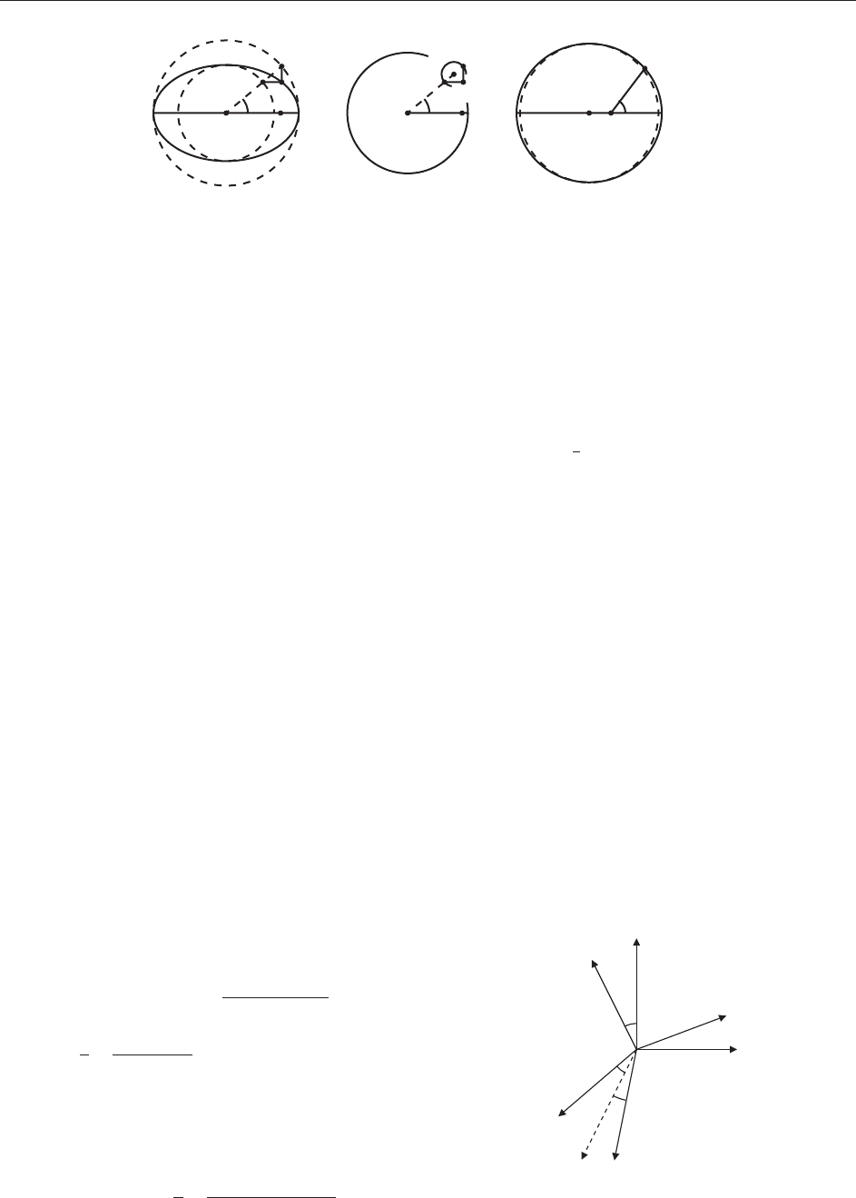
The eccentricity of the ellipse is e such that G =

L

ﬃﬃﬃﬃﬃﬃﬃﬃﬃﬃﬃﬃﬃ

1  e

. The ellipse equation is  = a(1 

e cos ), where  is the eccentric anomaly (see

Figure 2), a = L

=km

is the major semiaxis, and

 is the distance to the center of attraction S.

Finally, the relations between eccentric anomaly ,

average anomaly , true anomaly  (the latter is the

polar angle), and SP distance  are given by the

Kepler equations

 ¼   e sin 

ð1  e cos Þð1 þ e cos Þ¼1  e

 ¼ð1  e

3=2



d

ð1 þ e cos 



1  e

1 þ e cos 

½41

and the relation between true anomaly and average

anomaly can be inverted in the form

 ¼  þ g



 ¼  þ f



)



1  e

1 þ e cosð þ f



½42

where g



= g(e sin , e cos ), f



= f(e sin , e cos ),

and g(x, y), f (x, y) are suitable functions analytic

for jxj, jyj < 1. Furthermore, g(x, y) = x(1 þ y þ),

f (x, y) = 2x(1 þ

y þ) and the ellipses denote

terms of degree 2 or higher in x, y, containing only

even powers of x.

For more details, the reader is referred to Landau

and Lifshitz (1976) and Gallavotti (1983) .

Rigid Body

Another fundamental integrable system is the rigid

body in the absence of gravity and with a fixed point

O. It can be naturally described in terms of the Euler

angles 

, ’

(see Figure 3) and their derivatives



’

Let I

, I

be the three principal inertia moments

of the body along the three principal axes with unit

vectors i

, i

. The inertia moments and the

principal axes are the eigenvalues and the associated

unit eigenvectors of the 3  3 inertia matrix I,

which is defined by I

i = 1

)

, where

h, k = 1, 2, 3 and x

is the position of the ith particle

in a reference frame with origin at O and in which

e = 0.75

= 0.75

= 0.3

Figure 2 Eccentric and true anomalies of P, which moves on a small circle E centered at a point c moving on the circle D located

half-way between the two concentric circles containing the Keplerian ellipse: the anomaly of c with respect to the axis OS is . The

circle D is eccentric with respect to S and therefore  is, even today, called eccentric anomaly, whereas the circle D is, in ancient

terminology, the deferent circle (eccentric circles were introduced in astronomy by Ptolemy). The small circle E on which the point P

moves is, in ancient terminology, an epicycle. The deferent and the epicyclical motions are synchronous (i.e., they have the same

period); Kepler discovered that his key a priori hypothesis of inverse proportionality between angular velocity on the deferent and

distance between P and S (i.e., 

 = constant) implied both synchrony and elliptical shape of the orbit, with focus in S. The latter law is

equivalent to 

 = constant (because of the identity a

 = 

). Small eccentricity ellipses can hardly be distinguished from circles.

Figure 3 The Euler angles of the comoving frame i

, i

with

respect to a fixed frame x , y , z. The direction n is the ‘‘node line,

intersection between the planes x, y and i

, i

Introductory Article: Classical Mechanics 11

all particles are at rest: this comoving frame exists as

a consequence of the rigidi ty constraint. The

principal axes form a coordinate system which is

comoving as well: that is, in the frame (O; i

, i

)

as well, the particles are at rest.

The Lagrangian is simply the kinetic energy: we

imagine the rigidity constraint to be ideal (e.g., as

realized by internal central forces in the limit of

inf inite rigidity, as m entioned in the se ction ‘‘ Lag range

and Hamilton forms of equations of motion’’). The

angular velocity of the rigid motion is defined by

w ¼



n þ

’

z þ

½43

expressing that a generic infinitesimal motion

must consist of a variation of the three Euler

angles and, therefore, it has to be a rotation of

speeds



’

around the axes n, z, i

as shown

in Figure 3.

Let (!

, !

) be the components of w along the

principal axes i

, i

: for brevity, the latter axes

will often be called 1, 2, 3. Then the angular

momentum M, with respect to the pivot point O,

and the kinetic energy K can be checked to be

M ¼I

þ I

K ¼

ðI

þ I

½44

and are constants of motion. From Figure 3 it follows

that !



cos

’

sin

sin

, !

= 



sin

’

sin

cos

and !

’

cos

, so that the

Lagrangian, uninspiring at first, is

def



cos

’

sin 

sin

ð



sin

’

sin 

cos

’

cos 

½45

Angular momentum conservation does not imply

that the components !

are constants because

, i

also change with time according to

¼ w ^ i

; j ¼ 1; 2; 3

Hence,

M = 0 becomes, by the first of [44] and

denoting Iw = (I

, I

), the Euler equations

w þ w ^ Iw = 0,or

¼ðI

 I

Þ!

¼ðI

 I

Þ!

¼ðI

 I

Þ!

½46

which can be considered together with the conserved

quantities [44].

Since angular momentum is conserved, it is con-

venient to introduce the laboratory frame (O; x

, z

) with fixed axes x

, y

, z

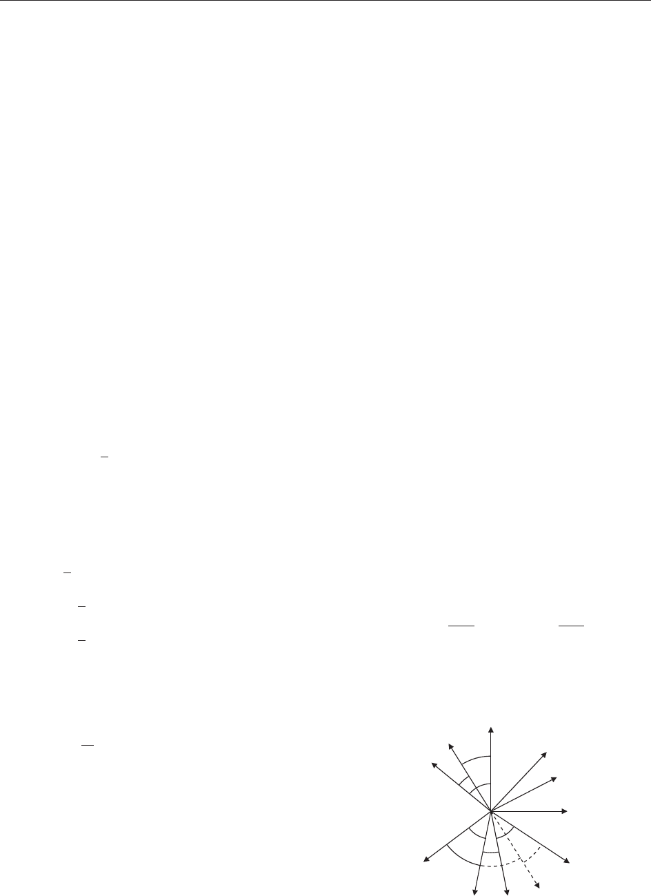
and (see Figure 4):

1. (O; x, y, z), the momentum frame with fixed axes,

but with z-axis oriented as M, and x-axis

coinciding with the node (i.e., the intersection)

of the x

–y

plane and the x–y plane (orthogonal

to M). Therefore, x, y, z is determined by the two

Euler angles ,  of (O; x, y, z)in(O; x

, y

, z

);

2. (O; 1, 2, 3), the comoving frame, that is, the

frame fixed with the body, and with unit vectors

, i

parallel to the principal axes of the body.

The frame is determined by three Euler angles



, ’

;

3. the Euler angles of (O; 1, 2, 3) with respect to

(O; x, y, z), which are denoted , ’, ;

4. G, the total angular momentum: G

;

5. M

, the angular momentum along the z

axis;

= G cos ; and

6. L, the projection of M on the axis 3, L = G cos .

The quantities G, M

, L, ’, , determine 

, ’

and



’

, or the p



, p

’

, p

variables

conjugated to 

, ’

as shown by the following

comment.

Considering Figure 4, the angle s ,  determine

location, in the fixed frame (O; x

, y

, z

) of the

direction of M and the node line m, which are,

respectively, the z-axis and the x-axis of the fixed

frame associated with the angular momentum ; the

angles , ’, then determine the position of the

comoving frame with respect to the fixed frame

(O; x, y, z), hence its position with respect to

(O; x

, y

, z

), that is, (

, ’

). From this and

G, it is possible to determine w because

cos  ¼

; tan ¼

¼I

2

ðG

 I

½47

and, from [43],



’

are determined.

x =m

||z

Figure 4 The laboratory frame, the angular momentum frame,

and the comoving frame (and the Deprit angles).

12 Introductory Article: Classical Mechanics

The Lagrangian [45] gives immediately (after

expressing w, i.e., n, z, i

, in terms of the Euler

angles 

, ’

) an expression for the variables



, p

’

, p

conjugated to 

, ’



¼ M n

; p

’

¼ M z

; p

¼ M i

½48

and, in principle, we could proceed to compute the

Hamiltonian.

However, the computation can be avoided

because of the very remarkable property (D

EPRIT),

which can be checked with some patience, making

use of [48] and of elementary spherical trigonometry

identities,

d þ G d’ þ L d

¼ p

’

d’

þ p



d

½49

which means that the map ((M

, ), (L, ),

(G, ’)) ! ((p



, 

), (p

’

, ’

), (p

)) is a canoni-

cal map. And in the new coordinates, the kinetic

energy, hence the Hamiltonian, takes the form

K ¼

þðG

 L

sin

cos

!"#

½50

This again shows that G, M

are constants of

motion, and the L, variables are determined by a

quadrature, because the Hamilton equation for

combined with the energy conservation yields

¼



sin



cos



ﬃﬃﬃﬃﬃﬃﬃﬃﬃﬃﬃﬃﬃﬃﬃﬃﬃﬃﬃﬃﬃﬃﬃﬃﬃﬃﬃﬃﬃﬃﬃﬃﬃﬃﬃﬃﬃﬃﬃﬃﬃﬃﬃﬃﬃﬃﬃ

2E  G

sin

cos





sin



cos

½51

In the integrability region, this motion is periodic

with some period T

(E, G). Once (t) is determined,

the Hamilton equation for ’ leads to the further

quadrature

’ ¼

sin

ðtÞ

cos

ðtÞ

G ½52

which determines a second periodic motion with

period T

(E, G). The , M

are constants and,

therefore, the motion takes place on three-

dimensional invariant tori T

E, G, M

in phase space,

each of which is ‘‘always’’ foliated into two-

dimensional invariant tori parametrized by the

angle  which is constant (by [50], because K is

-independent): the latter are in turn foliated by

one-dimensional invariant tori, that is, by periodic

orbits, with E, G such that the value of

(E, G)=T

(E, G) is rational.

Note that if I

= I

= I, the above analysis is

extremely simplified. Furthermore, if gravity g acts

on the system the Hamiltonian will simply change by

the addition of a potential mgz if z is the height of

the center of mass. Then (see Figure 4), if the center

of mass of the body is on the axis i

and z = h cos 

and h is the distance of the center of mass from O,

since cos 

= cos  cos   sin  sin  cos ’, the Hamil-

tonian will become H= K  mgh cos 

H¼

 L

mgh

 1 



1=2

 1 



1=2

cos ’

½53

so that, again, the system is integrable by quadratures

(with the roles of and ’ ‘‘interchanged’’ with respect

to the previous case) in suitable regions of phase space.

This is called the Lagrange’sgyroscope.

A less elementary integrable case is when the

inertia moments are related as I

= I

= 2I

and the

center of mass is in the i

–i

plane (rather than on

the i

-axis) and only gravity acts, besides the

constraint force on the pivot point O; this is called

Kowalevskaia’s gyroscope.

For more details, see Gallavotti (1983).

Other Quadratures

An interesting classical integrable motion is that of a

point mass attracted by two equal-mass centers of

gravitational attraction, or a point ideally constrained

to move on the surface of a general ellipsoid.

New integrable systems have been discovered

quite recently and have genera ted a wealth of new

developments ranging from group theory (as integ-

rable systems are closely related to symmetries) to

partial differential equations.

It is convenient to extend the notion of integ-

rability by stating that a system is integrable in a

region W of phase space if

1. there is a change of coordinates (p, q) 2

W ! {A, a, Y, y} 2 (U T

‘

)  (V  R

)where

U  R

‘

, V  R

,with‘ þ m  1, are open sets; and

2. the A, Y are constants of motion while the other

coordinates vary ‘‘linearly’’:

ða; yÞ!ða þ wðA; YÞt; y þ vðA; YÞtÞ½54

where w(A, Y), v(A, Y) are smooth functions.

In the new sense, the systems studied in the previous

sections are integrable in much wider regions (essen-

tially on the entire phase space with the exception of a

set of data which lie on lower-dimensional surfaces

Introductory Article: Classical Mechanics 13

forming sets of zero volume). The notion is con-

venient also because it allows us to say that even the

systems of free particles are integrable.

Two very remarkable systems integrable in the

new sense are the Hamiltonian systems, respectively

called Toda lattice (K

RUSKAL,ZABUSKY), and

Calogero lattice (C

ALOGERO,MOSER); if (p

, q

) 2 R

they are

ðp; qÞ¼

i¼1

n1

i¼1

g e

ðq

iþ1

q

ðp; qÞ¼

i¼1

i<j

ðq

 q

i¼1

½55

where m > 0 and , !, g  0. They describe the

motion of n interacting particles on a line.

The integration method for the above systems is

again to find first the constants of motion and later

to look for quadratures, when appropriate. The

constants of motion can be found with the method

of the Lax pairs. One shows that there is a pair of

self-adjoint n  n matrices M(p, q), N(p, q) such that

the equations of motion become

Mðp; qÞ¼i Mðp; qÞ; Nðp; qÞ½; i ¼

ﬃﬃﬃﬃﬃﬃﬃ

1

½56

which imply that M(t) = U( t)M(0)U(t)

1

,withU(t)a

unitary matrix. When the equations can be written in

the above form, it is clear that the n eigenvalues of the

matrix M(0) = M(p

, q

) are constants of motion.

When appropriate (e.g., in the Calogero lattice case

with !>0), it is possible to proceed to find canonical

action–angle coordinates: a task that is quite difficult

due to the arbitrariness of n, but which is possible.

The Lax pairs for the Calogero lattice (with

! = 0, g = m = 1) are

¼p

; N

¼ 0

ðq

 q

; N

ðq

 q

h 6¼ k

½57

while for the Toda lattice (with m = g =

 = 1) the

nonzero matrix elements of M, N are

¼ p

; M

h; hþ1

¼ M

hþ1; h

¼ e

ðq

q

hþ1

h; hþ1

¼N

hþ1; h

¼ ie

ðq

q

hþ1

½58

which are checked by first trying the case n = 2.

Another integrable system (S

UTHERLAND)is

ðp; qÞ¼

i¼k

h<k

sinh

ðq

 q

½59

whose Lax pair is related to that of the Calogero

lattice.

By taking suitable limits as n !1 and as the

other parameters tend to 0 or 1 at suitable rates,

integrability of a few differe ntial equations, among

which the Korteweg–deVries equation or the non-

linear Schro¨dinger equation, can be derived.

As mentioned in the introductory section, sym-

metry properties under continuous groups imply

existence of constants of motion. Hence, it is natural

to think that integrability of a mechanical system

reflects enough symmetry to imply the existence of

as many constants of motion, independent and in

involution, as the number of degree s of freedom, n.

This is in fact always true, and in some respects it

is a tautological statement in the anisochronous

cases. Integrability in a region W implies existence

of canonical action–angle coordinates (A, a) (see the

section ‘‘Quasi period icity and integrabi lity’’) an d the

Hamiltonian depends solely on the A’s: therefore, its

restriction to W is invariant with respect to the

action of the conti nuous commutative group T

the translations of the angle variables. The actions

can be seen as constants of motion whose existence

follows from Noether’s theorem, at least in the

anisochronous cases in which the Hamiltonian

formulation is equivalent to a Lagrangian one.

What is nontrivial is to recognize, prior to

realizing integrability, that a system admits this

kind of symmetry: in most of the interesting cases,

the systems either do not exhibit obvious symmetries

or they exhibit symmetries apparently unrelated to

the group T

, which nevertheless imply existence of

sufficiently many independent constants of motion

as required for integrability. Hence, nontrivial

integrable systems possess a ‘‘hidden’’ symmetry

under T

: the rigid body is an example.

However, very often the symmetries of a Hamiltonian

H which imply integrability also imply partial

isochrony, that is, they imply that the number of

independent frequencies is smaller than n (see the

section ‘‘Q uasiperi odicity and integrabi lity’’). Even

in such cases, often a map exists from the original

coordinates (p, q) to the integrating variables (A, a)

in whi ch A are constants of motion and the a are

uniformly rotating angles (some of which are also

constant) with spectrum w(A), whi ch is the gradient

h(A) for some function h(A) depending only on a

few of the A coordinates. However, the map might

fail to be canonical. The system is then said to be

bi-Hamiltonian: in the sense that one can represent

motions in two systems of canonical coordinates,

not related by a canonical transformation, and by

two Hamiltoni an functions H and H

 h which

generate the same motions in the respe ctive

14 Introductory Article: Classical Mechanics