Francoise J.-P., Naber G.L., Tsun T.S. (editors) Encyclopedia of Mathematical Physics

Подождите немного. Документ загружается.

This is a system describing a motion of a ‘‘pendu-

lum’’ ((p, q) coordinates) interacting with a ‘‘rotat-

ing wheel’’ ((A

, 

) coordinates) and a ‘‘clock’’

((A

, 

) coordinates) a priori unstable near the

points p = 0, q = 0, 2 (s

= 1, s

= 0, 

ﬃﬃﬃ

cf. [86]). It can be proved that on the energy surface

of energy E and for each " 6¼ 0 small enough (no

matter how small) there are initial data with action

coordinates close to A

= (A

, A

) with (1=2)A

þ A

close to E eventually evolving to a datum

= (A

, A

) with A

at a distance from A

smaller

than an arbitrarily prefixed distance (of course with

energy E). Furthermore, during the whole process

the pendulum energy stays close to zero within o(")

(i.e., the pendulum swings following closely the

unperturbed separatrices).

In other words, [90] describes a machine (the

pendulum) which, working approximately in a

cycle, extracts energy from a reservoir (the clock)

to transfer it to a mechanical device (the wheel). The

statement that diffusion is possible means that the

machine can work as soon as " 6¼ 0, if the initial

actions and the initial phases (i.e., 

, 

, p, q) are

suitably tuned (as functions of ").

The peculiarity of the system [90] is that the fixed

points P



of the unperturbed pendulum (i.e., the

equilibria p = 0, q = 0, 2) remain unstable equilibria

even when " 6¼ 0 and this is an important simplify-

ing feature.

It is a peculiarity that permits bypassing the

obstacle, arising in the analysis of more general

cases, represented by the resonance surfaces consist-

ing of the A’s with A



þ 

= 0: the latter

correspond to harmonics (

, 

) present in the

perturbing function, i.e., the harmonics whi ch

would lead to division by zero in an attempt to

construct (as necessary in studying [90] by Arnol’d’s

method) the parametric equations of the perturbed

invariant tori with action close to such A’s. In the

case of [90] the problem arises only on the

resonance marked in Figure 6 by a heavy line, i.e.,

= 0, corre sponding to cos 

in [90].

If " = 0, the points P



with p = 0, q = 0 and the

point P

with p = 0, q = 2 are both unstable

equilibria (and they are, of course, the same point,

if q is an angular variable). The unstable manifold

(it is a curve) of P

coincides with the stable

manifold of P



and vice versa. So that the

unperturbed system admits nontrivial motions lead-

ing from P

to P



and from P



to P

, both in a bi-

infinite time interval (1, 1): the p, q variables

describe a pendulum and P



are its unstable

equilibria which are connected by the separatrices

(which constitute the zero-energy surfaces for the

pendulum).

The latter property remains true for more general

a priori unstable Hamiltonians

¼H

ðAÞþH

ðp; qÞþ"f ðA; a; p; qÞ

in ðU T

‘

ÞðR

½91

where H

is a one-dimensional Hamiltonian which

has two unstable equilibrium points P

and P



linearly repulsive in one direction and linearly

attractive in another which are connected by two

heteroclinic trajectories which, as time tends to 1,

approach P



and P

and vice versa.

Actually, the points need not be different but, if

coinciding, the trajectories linking them must be

nontrivial: in the case [90] the variable q can be

considered an angle and then P

and P



would

coincide (but are connected by nontrivial trajec-

tories, i.e., by trajectories that also visit points

different from P



). Such trajectories are called

heteroclinic if P

6¼ P



and homoclinic if P

= P



In the general case, besides the homoclinicity (or

heteroclinicity) condition, certain weak genericity

conditions, automatically satisfied in the example

[90], have to be imposed in order to show that,

given A

and A

with the same unperturbed energy

E, one can find, for all " small enough but not equal

to zero, initial data ("-dependent) with actions

arbitrarily close to A

which evolve to data with

actions arbitrarily close to A

. This is a phenomenon

(a)

(b)

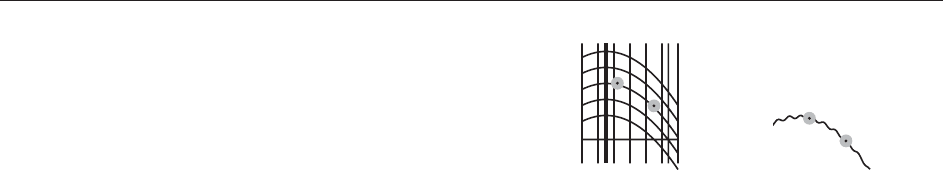
Figure 6 (a) The " = 0 geometry: the ‘‘partial energy’’ lines are

parabolas, (1=2)A

þ A

= const: The vertical lines are the

resonances A

= rational (i.e., 

þ 

= 0). The disks are

neighborhoods of the points A

and A

(the dots at their centers).

(b) " 6¼ 0; an artist’s rendering of a trajectory in A space, driven

by the pendulum swings to accelerate the wheel from A

to A

the expenses of the clock energy, sneaking through invariant tori

not represented and (approximately) located ‘‘away’’ from the

intersections between resonances and partial energy lines (a

dense set, however). The pendulum coordinates are not shown:

its energy stays close to zero, within a power of ". Hence the

pendulum swings, staying close to the separatrix. The oscilla-

tions symbolize the wiggly behavior of the partial energy

(1=2)A

þ A

in the process of sneaking between invariant tori

which, because of their invariance, would be impossible without

the pendulum. The energy (1=2)A

of the wheel increases

slightly at each pendulum swing: accurate estimates yield an

increase of the wheel speed A

of the order of "=( log "

1

)at

each swing of the pendulum implying a transition time of the

order of g

1=2

1

log "

1

Introductory Article: Classical Mechanics 25

called the Arnol’d diffusion. Simple sufficient con-

ditions for a transition from near A

to near A

are

expressed by the following result:

Theorem 7 Given the Hamiltonian [91] with H

admitting two hyperbolic fixed points P



with

heteroclinic connections, t !(p

(t), q

(t)), a = 1, 2,

suppose that:

(i) On the unperturbed energy surface of energy

E = H(A

) þH



) there is a regular curve

 : s !A(s) joining A

to A

such that the

unperturbed tori {A(s)}  T

‘

can be continued

at " 6¼ 0 into invariant tori T

A(s), "

for a set of

values of s which fills the curve  leaving only

gaps of size of order o(").

(ii) The ‘  ‘ matrix D

of the second derivatives of

the integral of f over the heteroclinic motions is

not degenerate, that is,

jdet Dj



det



1

dt @



f ðA; a þ wðAÞt;

ðtÞ; q

ðtÞÞ





> c > 0 ½92

for all A’s on the curve  and all a 2 T

Given arbitrary >0, for " 6¼ 0 small enough

there are initial data with action and energy closer

than  to A

and E, respectively, which after a long

enough time acquire an action closer than  to A

(keeping the initial energy).

The above two conditions can be shown to hold

generically for many pairs A

6¼ A

(and many

choices of the curves  connecting them) if the

number of degrees of freedom is 3. Thus, the result,

obtained by a simple extension of the argument

originally outlined by Arnol’d to discuss the para-

digmatic example [90], proves the existence of

diffusion in a priori unstable systems. The integral

in [92] is called Melnikov integral.

The real difficulty is to estimate the time needed

for the transition: it is a time that obv iously has to

diverge as " !0. Assuming g fixed (i.e., " indepen-

dent) a na ive approach easily leads to estimates

which can even be worse than O(exp (a"

b

)) with

some a, b > 0. It has finally been shown that in such

cases the minimum time can be, for rather general

perturbations "f (a, q), estimated above by

O("

1

log "

1

), which is the best that can be hoped

for under generic assumptions.

The reader is referred to Arnol’d (1989) and

Chierchi a and V aldinoci (2000) for more details.

Long-Time Stability of Quasiperiodic

Motions

A more difficult problem is whether the same

phenomenon of migration in action space occurs in

a priori stable systems. The root of the difficulty is a

remarkable stability property of quasiperiodic

motions. Consider Hamiltonians H

(A, a) = h(A) þ

"f (A, a) with H

(A) = h(A) strictly convex, analytic,

and anisochronous on the closure U of an open

bounded region U  R

‘

, and a perturbation "f (A, a)

analytic in

U  T

‘

Then a priori bounds are available on how long it

can possibly take to migrate from an action close to

to one close to A

: and the bound is of

‘‘exponential type’’ as " !0 (i.e., it admits a lower

bound which behaves as the exponential of an

inverse power of "). The simplest theorem is

EKHOROSSEV):

Theorem 7 There are constants 0 < a, b, d, g, 

such that any initial datum (A, a) evolves so that A

will not change by more than a"

before a long time

bounded below by  exp (b"

d

Thus, this puts an exponential bound, i.e., a

bound exponential in an inver se power of ", to the

diffusion time: before a time  exp (b"

d

) actions can

only change by O("

) so that their variation cannot

be large no matter how small " 6¼ 0 is chosen. This

places a (long) lower bound to the time of diffusion

in a priori stable systems.

The proof of the theore m provides, actually, an

interesting and detailed picture of the variations in

actions showing that some actions may vary more

slowly than others.

The theorem is constructive, i.e., all constants

0 < a, b, d,  can be explicitly chosen and depend

on ‘, H

, f although some of them can be fixed to

depend only on ‘ and on the minimum curvature of

the convex graph of H

. Its proof can be adapted

to cover many cases which do not fall in the class of

systems with strictly convex unperturbed Hamilto-

nian, and even to cases with a resonant unperturbed

Hamiltonian.

However, in important problems (e.g., in the

three-body problems met in celestial mechanics)

there is empirical evidence that diffusion takes

place at a fast pace (i.e., not exponentially slow in

the above sense) while the above results would

forbid a rapid migration in phase space if they

applied: however, in such problems the assumptions

of the theorem are not satisfied, because the

unperturbed system is strong ly resonant (as in the

celestial mechanics problems, where the number of

independent frequencies is a fraction of the number

26 Introductory Article: Classical Mechanics

of degrees of freedom and h(A) is far from strictly

convex), leaving wide open the possibility of observ-

ing rapid diffusion.

Further, changing the assumptions can dramati-

cally change the results. For instance, rapid diffusion

can sometimes be proved even though it might be

feared that it should require exponentially long

times: an example that has been proposed is the

case of a three-timescales system, with Hamiltonian

þ !

þ gð1 þ cos qÞ

þ "f ð

;

; p; qÞ½93

with w

def

, !

), where !

= "

1=2

!, !

= "

1=2

and

!>0 constants. The three scales are

1

ﬃﬃﬃﬃﬃﬃﬃ

1

, !

1

. In this case, there are many

(although by no means all) pairs A

, A

which can

be connected within a time that can be estimated to

be of order O("

1

log "

1

This is a rapid-diffusion case in an a priori

unstable system in which condition [92] is not

satisfied: because the "-dependence of w(A) implies

that the lower bound c in [92] must depend on "

(and be exponentially small with an inverse power

of " as " !0).

The unperturbed system in [93] is nonresonant in

the H

part for ">0 outside a set of zero measure

(i.e., where the vector w

satisfies a suitable

Diophantine property) and, furthermore, it is

a priori unstable: cases met in applicat ions can be

a priori stable and resonant (and often not aniso-

chronous) in the H

part. In such a system, not only

the speed of diffusion is not understood but

proposals to prove its existence, if present (as

expected), have so far not given really satisfactory

results.

For more details, the reader in referred

to Nekhorossev (1977).

The Three-Body Problem

Mechanics and the three-body problem can be

almost identified with each other, in the sense that

the motion of three gravitating masses has long been

a key astronomical problem and at the same time

the source of inspiration for many techniques:

foremost among them the theory of perturbations.

As an introduction, consider a special case. Let

three masses m

= m

, m

= m

, m

= m

interact

via gravity, that is, with interaction potential

km

 x

1

: the simplest problem arises

when the third body has a neg legible mass compared

to the two others and the latter are supposed to be

on a circular orbit; furthermore, the mass m

is "m

with " smal l and the mass m

moves in the plane of

the circular orbit. This will be called the ‘‘circular

restricted three-body problem.’’

In a refe rence system with center S and rotating at

the angular speed of J around S inertial forces

(centrifugal and Coriolis) act. Supposing that the

body J is located on the axis with unit vector i at

distance R from the origin S, the acceleration of the

point M is

€

R ¼ F þ!

R 

1 þ "



 2w

if F is the force of attraction and w

R  !

where w

is a vector with jw

j= !

and perpen-

dicular to the orbital plane and R

def

(

, 

)if

R = (

, 

). Here, taking into account that the origin

S rotates around the fixed center of mass, !

(R 

"R=(1 þ ")i) is the centrifugal force while 2w

is the Coriolis force. The equations of motion can

therefore be derived from a Lagrangian

L¼

 W þ !



R þ

 !

1 þ "

R  i ½94

with

¼ km

ð1 þ "Þ¼

def

W ¼

jRj



jR  Rij

where k is the gravitational constant, R the distance

between S and J, and finally the last three terms in [94]

come from the Coriolis force (the first) and from the

centripetal force (the other two, taking into account that

the origin S rotates around the fixed center of mass).

Setting g = g

=(1 þ ")  km

, the Hamiltonian of

the system is

H¼

ðp  !



jRj



 "

 i



1



 i



½95

The first part can be expressed immediately in the

action–angle coordinates for the two-body problem

(cf. the section ‘‘Newtonian potential and Kepler’s

laws’’). Calling such coordinates (L

, 

, G

, 

)and



the polar angle of M with respect to the major axis

of the ellipse and 

the mean anomaly of M on its

ellipse, the Hamiltonian becomes, taking into account

that for " = 0 the ellipse axis rotates at speed !

H¼

 !

 "

 i



1



 i



½96

Introductory Article: Classical Mechanics 27

which is convenient if we study the interior problem,

i.e., jRj < R. This can be expressed in the action–

angle coordinates via [41], [42]:



¼

þf



;

þ

¼

þ

þf



e ¼ 1 



1=2

;

jRj

1þecosð

þf



½97

where (see [42]), f



=f (esin, ecos) and

f ðx; yÞ¼2x 1 þ

y þ



with the ellipsis denoting higher orders in x, y even

in x. The Hamiltonian takes the form, if !

= gR

3

¼

!G

þ"

FðG

;

þ

Þ½98

where the only important feature (for our purposes) is

that F(L,G,,) is an analytic function of L,G,,

near a datum with jGj< L (i.e., e > 0) and jRj< R.

However, the domai n of analyticity in G is rather

small as it is constrained by jGj< L excluding in

particular the circular orbit case G = L.

Note that apparently the KAM theore m fails to be

applicable to [98] because the matrix of the second

derivatives of H

(L, G) has vanishing determinant.

Nevertheless, the proof of the theorem also goes

through in this case, with minor changes. This can

be checked by studying the proof or, following a

remark by Poincare´, by simply noting that the

‘‘squared’’ Hamiltonian H

def

)

has the form

¼

!G



þ"F

ðG

;

þ

Þ½99

with F

still analytic. But this time

det

@ðG

; L

¼6g

4

h 6¼ 0

if h ¼g

2

 2!G

6¼ 0

Therefore, the KAM theorem applies to H

and

the key observation is that the orbits generated by

the Hamiltonian (H

)

are geometrically the same as

those generated by the Hamiltonian H

: they are

only run at a different speed becau se of the need of a

time rescaling by the constant factor 2H

This shows that, given an unperturbed ellipse of

parameters (L

, G

) such that w = (g

, !),

> 0, with !

Diophantine, then the perturbed

system admits a motion which is quasiperiodic with

spectrum proportional to w and takes place on an orbit

which wraps around a torus remaining forever close to

the unperturbed torus (which can be visualized as

described by a point moving, according to the area law

on an ellipse rotating at a rate !

)withactions

, G

), provided " is small enough. Hence,

The KAM theorem answers, at least conceptually, the

classical question: can a solution of the three-body

problem remain close to an unperturbed one forever?

That is, is it possible that a solar system is stable

forever?

Assuming e, j%j=R 1 and retaining only the lowest

orders in e and j%j=R 1 the Hamiltonian [98]

simplifies into

H¼

!G

þ

ðG

Þ



3cos2ð

þ

e cos



e cosð

þ2

ecosð3

þ2



½100

where



ðG

Þ ¼ ðð1 þ "Þ

1=2

 1Þ!G



e ¼ 1 



1=2

It is an interesting exercise to estimate, assuming

as model the Hamiltonian [100] and following the

proof of the KAM theorem, how small has " to be if

a planet with the data of Mercury can be stable

forever on a (slowly precessing) orbit with actions

close to the present-day values under the influence

of a mass " times the solar mass orbiting on a circle,

at a distance from the Sun equal to that of Jupiter. It

is possible to follow either the above reduction to

the ordinary KAM theorem or to apply directly to

[100] the Lindstedt series expansion, proceeding

along the lines of the section ‘‘Quasip eriodicity and

KAM stability .’’ The first ap proach is easy but the

second is more efficient: in both cases, unless the

estimates are done in a particularly careful manner,

the value found for "m

is not interesting from the

viewpoint of astronomy.

The reader is refered to Arnol’d (1989) for more

details.

Rationalization and Regularization of

Singularities

Often integrable systems have interesting data which

lie on the boundary of the integrability domain. For

instance, the central motion when L = G (circular

orbits) or the rigid body in a rotation around one of

the principal axes or the two-body problem when

G = 0 (collisional data). In such cases, perturbation

28 Introductory Article: Classical Mechanics

theory cannot be applied as disc ussed abov e.

Typically, the perturbation depends on quantities

ﬃﬃﬃﬃﬃﬃﬃﬃﬃﬃﬃﬃﬃﬃ

L  G

and is not analytic at L = G. Never-

theless, it is sometimes possible to enlarge phase space

and introduce new coordinates in the vicinity of the

data which in the initial phase space are singular.

A notable example is the failure of the analys is of

the circular restricted three-body problem: it appar-

ently fails when the orbit that we want to perturb is

circular.

It is convenient to introduce the canonical

coordinates L,  and G, :

L ¼ L

; G ¼ L

 G

 ¼ 

þ 

;¼

½101

so that e =

ﬃﬃﬃﬃﬃﬃﬃﬃﬃﬃﬃﬃﬃﬃ

2GL

1

ﬃﬃﬃﬃﬃﬃﬃﬃﬃﬃﬃﬃﬃﬃﬃﬃﬃﬃﬃﬃﬃﬃﬃﬃﬃﬃ

1  G(2L)

1

and 

=  þ 

and 

= 

þ f



, where f



is defined in [42] (see

also [97]). Hence,



¼  þ  þ f

þ

;

þ 

¼  þ f

þ

e ¼

ﬃﬃﬃﬃﬃﬃﬃ

ﬃﬃﬃﬃﬃﬃﬃﬃﬃﬃﬃﬃﬃﬃﬃﬃﬃﬃﬃﬃﬃﬃﬃﬃﬃﬃ

1 



j%j

ð1  e

1 þ e cosð þ  þ f

þ

½102

and the Hamiltonian [100] takes the form

¼

 !L þ !G

þ "

FðL  G; L;þ ; Þ½103

In the coordinates L,G of [101] the unperturbed

circular case corresponds to G = 0 and [96], once

expressed in the action–angle variables G, L, , ,is

analytic in a domain whose size is controlled by

ﬃﬃﬃﬃﬃ

. Nevertheless, very often problems of perturba-

tion theory can be ‘‘regularized.’’

This is done by ‘‘enlarging the integrability’’

domain by adding to it points (one or more) around

the singularity (a boundary point of the domain of

the coordinates) and introducing new coordinates to

describe simultaneously the data close to the

singularity and the newly added points: in many

interesting cases, the equations of motion are no

longer singular (i.e., become analytic) in the new

coordinates and are therefore apt to describe the

motions that reach the singularity in a finite time.

One can say that the singularity was only apparent.

Perhaps this is best illustrated precisely in the

above circular restricted three-body problem, with

the singularity occurring where G = 0, that is, at a

circular unperturbed orbit. If we describe the points

with G small in a new system of coordinates

obtained from the one in [101] by letting alone

L,  and setting

p ¼

ﬃﬃﬃﬃﬃﬃﬃ

cos ; q ¼

ﬃﬃﬃﬃﬃﬃﬃ

sin  ½104

then p, q vary in a neighborhood of the origin with

the origin itself excluded.

Adding the origin of the p–q plane then in a full

neighborhood of the origin, the Hamiltonian [96] is

analytic in L, ,

p, q. This is because it is analytic

(cf. [96], [97]) as a function of L,  and e cos 

and of cos (

þ 

). Since 

=  þ  þ f

þ

and



þ 

=  þ f

þ

by [97], the Hamiltonian [96] is

analytic in L, , e cos ( þ  þ f

þ

), cos ( þ f

þ

)

for e small (i.e., for G small) and, by [42], f

þ

analytic in e sin ( þ ) and e cos ( þ ). Hence the

trigonometric identities

e sinð þ Þ¼

p sin  þ q cos 

ﬃﬃﬃﬃ

ﬃﬃﬃﬃﬃﬃﬃﬃﬃﬃﬃﬃﬃﬃﬃ

1 

e co sð þ Þ¼

p cos   q sin 

ﬃﬃﬃﬃ

ﬃﬃﬃﬃﬃﬃﬃﬃﬃﬃﬃﬃﬃﬃﬃ

1 

½105

together with G = (1=2)(p

þ q

) imply that [103] is

analytic near p = q = 0 and L > 0,  2 [0, 2]. The

Hamiltonian becomes analytic and the new coordi-

nates are suitable to describe motions crossing the

origin: for example, by setting

C ¼

def

1 

þ q



1=2

[100] becomes

H¼

 !L þ !

ðp

þ q

þ 

ðp

þ q

ÞÞ 

ðL 

ðp

þ q

ÞÞ

ð3 cos 2  ðð11 cos  þ 3 cos 3Þp

ð7 sin  þ 3 sin 3ÞqÞCÞ½106

The KAM theorem does not apply in the form

discussed above to ‘‘Cartesian coordinates,’’ that is,

when, as in [106], the unperturbed system is not

assigned in action–angle variables. However, there

are versions of the theorem (actually its corollaries)

which do apply and therefore it becomes possible to

obtain some results even for the perturbations of

circular motions by the techniques that have been

illustrated here.

Likewise, the Hamiltonian of the rigid body with

a fixed point O and subject to analytic external

forces becomes singular, if expressed in the action–

angle coordinates of Depr it, when the body motion

nears a rotation around a principal axis or, more

generally, nears a configuration in which any two of

Introductory Article: Classical Mechanics 29

the axes i

, z,orz

coincide (i.e., any two among the

principal axis, the angular momentum axis a nd the

inertial z-axis coincide; see the section ‘‘Rigid

body’’). Nevertheless, by imitating the procedure

just described in the simpler cases of the circular

three-body problem, it is possible to enlarge the

phase space so that in the new coordinates the

Hamiltonian is analytic near the singular

configurations.

A regularization also arises when considering

collisional orbits in the unrestricted planar three-

body problem. In this respect, a very remarkable

result is the regularization of collisional orbits in the

planar three-body problem. After proving that if the

total angular momentum does not vanish, simulta-

neous collisions of the three masses cannot occur

within any finite time interval, the question is

reduced to the regularization of two-body collisions,

under the assumption that the total angular momen-

tum does not vanish.

The local change of coordinates, which changes the

relative position coordinates (x, y) of two colliding

bodies as (x, y) !(, ), with x þ iy = ( þ i)

, is not

one to one, hence it has to be regarded as an

enlargement of the positions space, if points with

different (, ) are considered different. However, the

equations of motion written in the variables ,  have

no singularity at ,  = 0(L

EVI-CIVITA).

Another celebrated regularization is the regular-

ization of the Sch wartzschild metric, i.e., of the

general relativity version of the two-body problem:

it is, however, somewhat out of the scope of this

review (S

YNGE,KRUSKAL).

For more details, the reader is refered to Levi-

Civita (1956).

Appendix 1: KAM Resummation Scheme

The idea to control the ‘‘remaining contributions’’ is to

reduce the problem to the case in which there are no

pairs of lines that follow each other in the tree order

and which have the same current. Mark by a scale

label ‘‘0’’ the lines, see [74], [83], of a tree whose

divisors C=w

:n(l)are>1: these are lines which give

no problems in the estimates. Then mark by a scale

label ‘‘1’’ the lines with current n(l) such that

 n(l)j2

nþ1

for n = 1 (i.e., the remaining lines).

The lines labeled 0 are said to be on scale 0, while

those labeled 1 are said to be on scale 1. A cluster

of scale 0 will be a maximal collection of lines of

scale 0 forming a connected subgraph of a tree .

Consider only trees 

2 

of the family 

trees containing no cluster s of lines with scale label

0 which have only one line entering the cluster and

one exiting it with equal current.

It is useful to introduce the notion of a line ‘

situated ‘‘between’’ two lines ‘, ‘

with ‘

>‘: this

will mean that ‘

precedes ‘

but not ‘.

All trees  in which there are some pairs l

> l of

consecutive lines of scale label 1 which have equal

current and such that all lines between them bear

scale label 0 are obtained by ‘‘inserting’’ on the lines

of trees in 

with label 1 any number of clusters

of lines and nodes, with lines of scale 0 and with the

property that the sum of the harmonics of the nodes

inserted vanishes.

Consider a line l

2

2 

linking nodes v

< v

and labeled 1 and imagine inserting on it a cluster

 of lines of scale 0 with sum of the node harmonics

vanishing and out of which emerges one line

connecting a node v

out

in  to v

and into which

enters one line linking v

to a node v

2 . The

insertion of a k–lines, jj= (k þ 1)-nodes, cluster

changes the tree value by replacing the line factor,

that will be briefly called ‘‘value of the cluster ’’, as

 n

 nðl

ðn

Mð; nðl

ÞÞn

 nðl

½107

where M is an ‘  ‘ matrix

ð;nðl

ÞÞ ¼

jj



out; r



in; s

v2

ðf

l2

 n

 nðlÞ

if ‘ = v

v denotes a line linking v

and v. Therefore, if

all possible connected clusters are inserted and the

resulting values are added up, the result can be taken

into account by attributing to the original line l

factor like [107] with M

(0)

(n(l

)) =

def



M(; n(l

))

replacing M(; n(l

)).

If several connected clusters  are inserted on the

same line and their values are summed, the result is

a modification of the factor associated with the line

into

k¼0



ð0Þ

ðnðl

ÞÞ

 nðl

¼ n



 nðl

 M

ð0Þ

ðnðl

ÞÞ

½108

The series defining M

(0)

involves, by construction, only

trees with lines of scale 0, hence with large divisors, so

that it converges to a matrix of small size of order "

(actually "

, more precisely) if " is small enough.

Convergence can be established by simply remark-

ing that the series defining M

(1)

is built with lines

with values >(1=2) of the propagator, so that it

certainly converges for " small enough (by the

estim ates in the section ‘‘Perturbi ng funct ions,’’

where the propagators were ident ically 1) and the

30 Introductory Article: Classical Mechanics

sum is of order " (actually "

), hence <1. However,

such an argument cannot be repeated when dealing

with lines with smaller propagators (which still have

to be discussed). Therefore, a method not relying on

so trivial a remark on the size of the propagators has

eventually to be used when considering lines of scale

higher than 1, as it will soon become neces sary.

The advantage of the collection of terms achieved

with [108] is that we can represent h as a sum of

values of trees which are simpler because they

contain no pair of lines of scale 1withinbetween

lines of scale 0 with total sum of the node harmonics

vanishing. The price is that the divisors are now more

involved and we even have a problem due to the fact

that we have not proved that the series in [108]

converges. In fact, it is a geometric series whose value

is the RHS of [108] obtained by the sum rule [79]

unless we can prove that the ratio of the geometric

series is <1. This is trivial in this case by the previous

remark: but it is better to note that there is another

reason for convergence, whose use is not really

necessary here but will become essential later.

The property that the ratio of the geometric series

is <1 can be regarded as due to the consequence of

the cancell ation mentione d in the section ‘‘Q uasi-

perio dicity an d KAM stability ’’ which can be

shown to imply that the ratio is <1 because

(0)

(n) = "

 n)

(0)

(n) with C jm

(0)

(n)j< D

for some D

> 0 and for all j"j <"

for some "

Then for small " the divisor in [108] is essentially

still what it was before starting the resummation.

At this point, an induction can be started. Consider

trees evaluated with the new rule and place a scale

level ‘ ‘2’ ’ on the lines with C jw

 n(l)j2

nþ1

for

n = 2: leave the label ‘ ‘0’’ on the lines already marked

so and label by ‘ ‘1’’ the other lines. The lines of scale

‘ ‘1’’ will satisfy 2

n

< jw

 n(l)j2

nþ1

for n = 1.

The graphs will now possibly contain lines of scale 0,

1or2 while lines with label ‘ ‘1’’ no longer can

appear, by construction.

A cluster of scale 1 will be a maximal collection of

lines of scales 0, 1 forming a connected subgraph of

a tree  and containing at least one line of scale 1.

The construction carried out by considering clusters

of scale 0 can be repeated by considering trees 

2 

with 

the collection of trees with lines marked 0, 1,

or 2 and in which no pairs of lines with equal

momentum appear to follow each other if between

them there are only lines marked 0 or 1.

Insertion of connected clusters  of such lines on a

line l

of 

leads to define a matrix M

(1)

formed by

summing tree values of clusters  with lines of scales

0 or 1 evaluated with the line fact ors defined in

[107] and with the restriction that in  there are no

pairs of lines ‘<‘

with the same current and which

follow each other while any line between them has

lower scale (i.e., 0), here ‘‘between’’ means ‘‘preced-

ing l

but not preceding l,’’ as above.

Therefore, a scale-independent method has to be

devised to check the convergence for M

(1)

and for the

matrices to be introduced later to deal with even

smaller propagators. This is achieved by the following

extension of Siegel’s theorem mentioned in the section

‘‘Quasiperiodicity and KAM stability’’:

Theorem 8 Let w

satisfy [74] and set w = Cw

Consider the contribution to the sum in [82] from

graphs  in which

(i) no pairs ‘

>‘ of lines which lie on the same

path to the root carry the same current n if all

lines ‘

between them have current n(‘

) such

that jw  n(‘

)j > 2jw  nj;

(ii) the node harmonics are bounded by jnjN for

some N.

Then the number of lines ‘ in  with divisor w  n

‘

satisfying 2

n

< jw  n

‘

j2

nþ1

does not exceed

4 Nk2

n=

, n = 1, 2, ....

This implies, by the same estimates in [85], that

the series defining M

(1)

converges. Again, it must be

checked that there are cancellations implying that

(1)

(n) = "

 n)

(1)

(n) with jm

(1)

(n)j < D

for

the same D

> 0 and the same "

At this point, one deals with trees containing only

lines carrying labels 0, 1, 2, and the line factors for

the lines ‘ = v

v of scale 0 are n

n

=(w

n(‘))

those of the lines ‘ = v

v of scale 1 have line factors

(w

n(‘)

 M

(0)

(n(‘)))

1

, and those of the

lines ‘ = v

v of scale  2 have line factors

ðw

 nð‘Þ

 M

ð1Þ

ðnð‘ÞÞÞ

1

Furthermore, no pair of lines of scale ‘‘1’’ or of scale

‘‘2’’ with the same momentum and with only lines

of lower scale (i.e., of scale ‘‘0’’ in the first case or of

scale ‘‘0’’, ‘‘1’’ in the second) between them can

follow each other.

This procedure can be iterated until, after infi-

nitely many steps, the problem is reduced to the

evaluation of tree values in which each line carries a

scale label n and there are no pairs of lines which

follow each other and which have only lines of

lower scale in between. Then the Siegel argument

applies once more and the series so resumed is an

absolutely convergent series of functions analytic in

": hence the original series is convergent.

Although at each step there is a lower bound on the

denominators, it would not be possible to avoid using

Siegel’s theorem. In fact, the lower bound would become

worse and worse as the scale increases. In order to check

Introductory Article: Classical Mechanics 31

the estimates of the constants D

, "

which control the

scale independence of the convergence of the various

series, it is necessary to take advantage of the theorem,

and of the absence (at each step)ofthenecessityof

considering trees with pairs of consecutive lines with

equal momentum and intermediate lines of higher scale.

One could also perform the analysis by bounding

(k)

order by order with no resummations (i.e.,

without changing the line factors) and exhibiting the

necessary cancellations. Alternatively, the paths that

Kolmogorov, Arnol’ d and Moser used to prove

the first three (somewhat differen t) versions of the

theorem, by successive approximations of the

equations for the tori, can be followed.

The invariant tori are Lagrangian manifolds just

as the unperturbed ones (cf. comments after [31])

and, in the case of the Hamiltonian [80], the

generating function A  y þ (A, y ) can be

expressed in terms of their parametric equations

ðA; y Þ¼Gðy Þþa  y þhðy ÞðA w  hðy ÞÞ

Gðy Þ¼

def

hðy Þþh



ðy Þ¶

h



ðy Þa

a ¼

def

ðhðy Þþh



ðy Þ¶

h



ðy ÞÞ

ð2Þ

‘



ðy Þ¶

h



ðy Þ

ð2Þ

‘

½109

where =(w ¶

) and the invariant torus corre-

sponds to A

= w in the map a = y þ¶

F(A, y ) and

= A þ ¶

(A, y ). In fact, by [109] the latter

becomes A

= A  h and, from the second of [75]

written for f depending only on the angles a,itis

A = w þh when A, a are on the invariant torus.

Note that if a exists it is necessarily determined by the

third relation in [109] but the check that the second

equation in [109] is soluble (i.e., that the RHS is an exact

gradient up to a constant) is nontrivial. The canonical

map generated by A  y þ F(A, y ) is also defined for A

close to w and foliates the neighborhood of the invariant

torus with other tori: of course, for A

6¼ w the tori

defined in this way are, in general, not invariant.

The reader is referred to Gallavotti et al. (2004)

for more details.

Appendix 2: Coriolis and Lorentz

Forces – Larmor Precession

Larmor precessio n refers to the motion of an

electrically charge d particle in a magnetic field H

(in an inertial frame of reference). It is due to the

Lorentz force which, on a unit mass with unit

charge, produces an acceleration

€

R = v ^ H if the

speed of light is c = 1.

Therefore, if H = Hk is directed along the k-axis,

the acceleration it pr oduces is the same that the

Coriolis force would impress on a unit mass located

in a reference frame which rotates with angular

velocity !

k around the k-axis if H = 2!

The above remarks imply that a homogeneous

sphere electrically charged uniformly with a unit

charge and freely pivoting about its center in a

constant magnetic field H dire cted along the k-axis

undergoes the same motion as it would follow if not

subject to the magnetic field but seen in a

noninertial reference frame rotating at constant

angular velocity !

around the k-axis if H and !

are related by H = 2!

: in this frame, the Coriolis

force is interpreted as a magnetic field.

This holds, however, only if the centrifugal force

has zero moment with respect to the center: true in

the spherical symmetry case only. In spherically

nonsymmetric cases, the centrifugal forces have in

general nonzero moment, so the equivalence

between Coriolis force and the Lorentz force is

only approximate.

The Larmor theorem makes this more precise. It

gives a quantitative estimate of the difference between

the motion of a general system of particles of mass m

in a magnetic field and the motion of the same

particles in a rotating frame of reference but in the

absence of a magnetic field. The approximation is

estimated in terms of the size of the Larmor frequency

eH=2mc, which should be small compared to the

other characteristic frequencies of the motion of the

system: the physical meaning is that the centrifugal

force should be small compared to the other forces.

The vector potential A for a constant magnetic

field in the k-direction, H = 2!

k,isA = 2!

k ^ R 

. Therefore, from the treatment of the Coriolis

force in the sect ion ‘‘Three -body prob lem’’ (see

[95]), the motion of a charge e with mass m in a

magnetic field H with vector potential A and subject

to other forces with potential W can be described, in

an inertial frame and in generic units, in which the

speed of light is c, by a Hamiltonian

H¼

p 



þWðRÞ½110

where p = m

R þ (e=c)A and R are canonically con-

jugate variables.

Further Reading

Arnol’d VI (1989) Mathematical Methods of Classical Mechanics.

Berlin: Springer.

Calogero F and Degasperis A (1982) Spectral Transform and

Solitons. Amsterdam: North-Holland.

32 Introductory Article: Classical Mechanics

Chierchia L and Valdinoci E (2000) A note on the construction of

Hamiltonian trajectories along heteroclinic chains. Forum

Mathematicum 12: 247–255.

Fasso` F (1998) Quasi-periodicity of motions and complete

integrability of Hamiltonian systems. Ergodic Theory and

Dynamical Systems 18: 1349–1362.

Gallavotti G (1983) The Elements of Mechanics. New York:

Springer.

Gallavotti G, Bonetto F, and Gentile G (2004) Aspects of the

Ergodic, Qualitative and Statistical Properties of Motion.

Berlin: Springer.

Kolmogorov N (1954) On the preservation of conditionally

periodic motions. Doklady Akademia Nauk SSSR 96:

527–530.

Landau LD and Lifshitz EM (1976) Mechanics. New York:

Pergamon Press.

Levi-Civita T (1956) Opere Matematiche. Accademia Nazionale

dei Lincei. Bologna: Zanichelli.

Moser J (1962) On invariant curves of an area preserving

mapping of the annulus. Nachricten Akademie Wissenschaften

Go¨ ttingen 11: 1–20.

Nekhorossev V (1977) An exponential estimate of the time of

stability of nearly integrable Hamiltonian systems. Russian

Mathematical Surveys 32(6): 1–65.

Poincare´ H (1987) Me´thodes nouvelles de la me´canique cele`ste

vol. I. Paris: Gauthier-Villars. (reprinted by Gabay, Paris,

1987).

Introductory Article: Differential Geometry

S Paycha, Universite

Blaise Pascal, Aubie

re, France

Differential geometry is the study of differential

properties of geometric objects such as curves,

surfaces and higher-dimensional manifolds endowed

with additional structures such as metrics and

connections. One of the main ideas of differential

geometry is to apply the tools of analysis to

investigate geometric problems; in particular, it

studies their ‘‘infinitesimal parts,’’ thereby lineariz-

ing the problem. However, historically, geometric

concepts often anticipated the analytic tools

required to define them from a differential geometric

point of view; the notion of tangent to a curve, for

example, arose well before the notion of derivative.

In its barely more than two centurie s of existence,

differential geometry has always had strong (often

two-way) interactions wi th physics. Just to name a

few examples, the theory of curves is used in

kinematics, symplectic manifolds arise in Hamilto-

nian mechanics, pseudo-Riemannian manifolds in

general rel ativity, spinors in quantum mech anics, Lie

groups and principal bundles in gauge theory, and

infinite-dimensional manifolds in the path-integral

approach to quantum field theory.

Curves and Surfaces

The study of differential properties of curves and

surfaces resulted from a combination of the coordi-

nate method (or analytic geometry) developed by

Descartes and Fermat during the first half of the

seventeenth century and infinitesimal calculus devel-

oped by Leibniz and Newton during the second half

of the seventeenth and beginning of the eighteenth

century.

Differential geometry appeared later in the eight-

eenth century with the works of Euler Recherches

sur la courbure des surfaces (1760) (Investigations

on the curvature of surfaces) and Monge Une

application de l’analyse a`lage´ome´trie (1795) (An

application of analysis to geometry). Until Gauss’

fundamental article Disquisitiones generales circa

superficies curvas (General investigations of curved

surfaces) published in Latin in 1827 (of which one

can find a partial translation to English in Spivak

(1979)), su rfaces embedded in R

were either

described by an equation, W(x, y, z) = 0, or by

expressing one variable in terms of the others.

Although Euler had already noticed that the

coordinates of a point on a surface could be

expressed as functions of two independent variables,

it was Gauss who first made a systematic use of such

a parametric representation, thereby ini tiating the

concept of ‘‘local chart’’ which underlies differe ntial

geometry.

Differentiable Manifolds

The actual notion of n-manifold independent of a

particular embedding in a Euclidean space goes back

to a lecture U

ber die Hypothesen, welche der

Geometrie zu Grunde liegen (On the hypotheses

which lie at the foundations of geometry) (of which

one can find a translation to English and comments

in Spivak (1979)) delivered by Riemann at Go¨ ttingen

University in 1854, in which he makes clear the

fact that n-manifolds are locally like n-dimensional

Euclidean space. In his work, Riemann mentions

the existence of infinite-dimensional manifolds,

such as function spaces, which today play an

important role since they naturally arise as config-

uration spaces in quantum field theories.

In modern language a differentiable manifold

modeled on a topolog ical space V (which can be

Introductory Article: Differential Geometry 33

finite dimensional, Fre´chet, Banach, or Hilbert for

example) is a topological space M equipped with a

family of local coordinate charts (U

, 

)

i2I

such that the

open subsets U

 M cover M and where 

: U

! V,

i 2 I, are homeomorphisms which give rise to smooth

transition maps 

 

1

: 

\ U

) ! 

\ U

An n-dimensional differentiable manifold is a differ-

entiable manifold modeled on R

. The sphere

n1

:= {(x

, ..., x

) 2 R

i = 1

= 1} is a differenti-

able manifold of dimension n  1.

Simple differentiable curves in R

are one-

dimensional differentiable manifolds locally speci-

fied by coordinates x(t) = (x

(t), ..., x

(t)) 2 R

where t 7!x

(t) is of class C

. The tangent at point

x(t

) to such a curve, which is a straight line passing

through this point with direction given by the vector

), generalizes to the concept of tangent space

M at point m 2 M of a smooth manifold M

modeled on V which is a vector space isomorphic to

V spanned by tangent vectors at point m to curves

(t) of class C

on M such that (t

) = m.

In order to make this more precise, one needs the

notion of differentiable mapping. Given two differ-

entiable manifolds M and N, a mapping f : M ! N

is differentiable at point m if, for every chart (U , )

of M containing m and every chart (V, )ofN such

that f (U)  V,themapping  f  

1

: (U) ! (V)

is differentiable at point (m). In particular, differenti-

able mappings f : M ! R form the algebra C

(M, R)

of smooth real-valued functions on M. Differentiable

mappings  :[a, b] ! M from an interval [a, b]  R to

a differentiable manifold M are called ‘‘differentiable

curves’’ on M. A differentiable mapping f : M ! N

which is invertible and with differentiable inverse

1

: N ! M is called a diffeomorphism.

The derivative of a function f 2 C

(M, R) along

acurve :[a, b] ! M at point (t

) 2 M with t

[a, b]isgivenby

Xf :¼

t¼t

f  ðtÞ

and the map f 7!Xf is called the tangent vector to

the curve  at point (t

). Tangent vectors to some

curve  :[a, b] ! M at a given point m 2 ([a, b])

form a vector space T

M called the ‘‘tangent space’’

to M at point m.

A (smooth) map which, to a point m 2 M, assigns

a tangent vector X 2 T

M is called a (smooth)

vector field. It can also be seen as a derivation

X : f 7!Xf on C

(M, R) defined by (

Xf )(m):=

X(m)f for any m 2 M and the bracket of vector

fields is thereby defined from the operator bracket

[X, Y]:=

X 

Y 

Y 

X. The linear operations on

tangent vectors carry out to vector fields (X þ

Y)(m):= X(m) þ Y(m), (X)(m):= X(m) for any

m 2 M and for any X, Y 2 T

M,  2 R so that

vector fields on M build a linear space.

One can generate tangent vectors to M via local

one-parameter groups of differentiable transforma-

tions of M, that is, mappings (t, m) 7!

(m) from

], [  U to U (with >0 and U  M an

open subset of M) such that 

= Id, 

tþs

= 

 

8s, t 2 ], [ with t þ s 2 ], [ and m 7!

(m)isa

diffeomorphism of U onto an open subset 

(U).

The tangent vector at t = 0 to the curve (t ) = 

(m)

yields a tangent vector to M at point m = (0).

Conversely, when M is finite dimensional, the

fundamental theorem for systems of ordinary

equations yields, for any vector field X on M, the

existence (around any point m 2 M)ofa

local one-parameter group of local transformations

 :], [  U !M (with U an open subset contain-

ing m) which induces the tangent vector

X(m) 2 T

A differentiable mapping  : M !N induces a map





(m):T

M !T

(m)

M defined by 



Xf = X(f  ).

An ‘ ‘immersion’’ of a manifold M in a manifold N is a

differentiable mapping  : M !N such that the maps





(m) are injective at any point m 2 M.Suchamapis

an embedding if it is moreover injective in which case

(M)  N is a submanifold of N. The unit sphere S

is a submanifold of R

nþ1

. Whitney showed that every

smooth real n-dimensional manifold can be embedded

in R

2nþ1

A differentiable manifold whose coordinate charts

take values in a complex vector space V and whose

transition maps are holomorphic is called a complex

manifold, which is complex n-dimensional if V = C

The complex projective space CP

,theunionof

complex straight lines through 0 in C

nþ1

,isa

compact complex manifold of dimension n. Similarly

to the notion of differentiable mapping between

differentiable manifolds, we have the notion of

holomorphic mapping between complex manifolds.

A smooth family m 7!J

of endomorphisms of the

tangent spaces T

M to a differentiable manifold M such

that J

= Id gives rise to an almost-complex manifold.

The prototype is the almost-complex structure on C

defined by J(@

) = @

; J(@

) = @

with z = (x

, ..., x

þ iy

) 2 C

which can be transferred to a

complex manifold M by means of local charts. An

almost-complex structure J on a manifold M is called

complex if M is the underlying differentiable manifold

of a complex manifold which induces J in this way.

Studying smooth functions on a differentiable

manifold can provide information on the topology

of the manifold: for example, the behavior of a

smooth function on a compact manifold as its

critical points strongly restricted by the topological

properties of the manifold. This leads to the Morse

34 Introductory Article: Differential Geometry