Francoise J.-P., Naber G.L., Tsun T.S. (editors) Encyclopedia of Mathematical Physics

Подождите немного. Документ загружается.

According to the proposal of Hartle and Hawking,

one adopts path-integral formalism for the Eucli-

dean action where the functional integral is not only

carried out over the 4-metric, g



, and the scalar

field , but also one takes sum over the class of

manifolds, M. Note that B is a part of the bounda ry

of this set of manifold. If



and



 are the induced

metric and the configuration of the scalar field, ,

on the boundary, B, then the propagator (henceforth

we just call it the wave function) [



, B] can be

given a functional-integral representation. Indeed,

obtaining the most general form of the path integral,

summing over the 4-manifolds, is quite a formidable

task. On the other hand, if one chooses a class of

4-manifolds which can be decomposed as a product

(foliation) R  B, the wave function is expressed as

½



; B



D f ðN



Þ

S

½g



;

½26

We have introduced the gauge-fixing condition

as f (N



), which is usually taken to be



= l



and

then the corresponding Faddeev–Popov determinant,



, has to be inserted into the path-integral

measure. We recall from our earlier discussions

that N



has to be unrestricted on the boundary, B,

since they have no dynamical role when we express

the action in terms of the variables defined on the

3-surface. As noted in the previous discussion,

explicit time dependence does not appear after the

3 þ 1 split and (h

(x), (x)) ha ve no dependence on

t. Therefore, we introduce a parameter to designate

the paths over which the functional integral is to be

taken. Recall that in the quantum-mechanical case,

the paths are parametrized as q

(t) for the coordi-

nates. However, when we resort to a parametriza-

tion of the variables for the case at hand, certain

conditions must be fulfilled. We are permitted to

integrate over h

and  over only those paths, while

parametrizing them as (h

(x, ), (x, )), so that they

match the arguments of the wave function on the

boundary B. Therefore, we may define the metric

and the scalar field configuration so that at  = 1

they assume their functional values on the boundary:

in other words,



(x) = h

(x,  = 1) and



(x) = (x,  = 1). It is worthwhile to go back to

the quantum-mechanical analogy once more. When

we compute amplitudes/propagators in quantum

mechanics, the functional integral is defined for the

amplitude of going from a configuration q

to q

while summing over all possible paths originating

from one endpoint q

and ending at the final point

. On this occasion, we have imposed the con-

straint on the final endp oint belonging to the

boundary B. Thus, in order to determine the wave

function of the universe, we are required to specify

the initial configurations of h

and  at  = 0. We

shall not enter into important issues related with the

properties of the Euclidean action, the problems

associated with the choice of contours of the path

integrals, and related topics. The reader will find

detailed discussions in the lectures and monographs

referre d in the ‘‘Furt her readi ng’’ section.

It is important to re-emphasize that boundary

conditions are to be introduced while solving the

WDW equation. It was argued by De Witt that the

wave function will be determined uniquely from the

mathematical consistency of the theory and that

hope has not been realized. Whether one attempts to

solve the functional differential WDW equation or

obtain the wave function in the path-integral

formalism, the issue of boundary condition is

unavoidable. There are mainly three differe nt kinds

of boundary conditions in quantum cosmology:

Hartle–Hawking (HH) no-boundary proposal,

Vilenkin’s tunneling mechanism, and Linde’s bound-

ary condition. We shall briefly discuss the first two

proposals. Instead of stating the boundary condi-

tions in full generality, we shall envisage quantum

cosmology in a minisuperspace and provide illus-

trative examples to compare the main features of

HH and Vilenkin solutions to the WDW equation.

It is realized that the discussion and solutions of

quantum cosmology in the superspace is rather

difficult, since we deal with functional differential

equations and the configuration space is infinite

dimensional. Therefore, it is worthwhile to consider

a syst em, as a simple model, which has finite degrees

of freedom. Thus, we assume that the metric and

matter fields depend only on cosmic time to begin

with. There is a physical motivation behind this

assumption, since the present classical state of the

universe is described by the Friendmann–Robertson–

Walker (FRW) metric corresponding to an isotropic

and homogeneous universe. Notice that the classical

evolution equation resembles that of the motion of a

particle. The quantum evolution equations are now

given by differential equations of quantum

mechanics rather than functional differential equa-

tions. Similarly, the path-integral formulation

becomes analogous to the quantum-mechanical

frame work. Of course, adopting such a simplified

approach deprives us from describing some of the

important aspects of quantum gravity. However,

within this framework, several essential features can

be exhibited and deep insight might be gained into

the physics of the very early universe. The first step

in getting the minisuperspace metric is to assume

that the lapse is homogeneous, that is, N

= N

(t)

458 Wheeler–De Witt Theory

and the shift is set to zero, N

= 0. Thus, the metric

takes the form

¼ðN

ðtÞÞ

þ h

ðx; tÞdx

½27

The relevant choice of 3-metric for FRW isotropic

and homogeneous universe is

ðx; tÞdx

¼ aðtÞ

d

½28

Note that d

is the metric on a 3-sphere. It is

straightforward to derive the Friedmann equations

for such a geometry.

The HH no-boundary condition can be inter-

preted as a topological proposition about the set of

path over which we have to sum. The 3-surface B is

to be taken as the only surface of compact

4-manifold M which is endowed with the metric



, and



and



 are the induced metric and the

scalar field on the surface. The wave function is

obtained by using the matching condition supple-

mented with initial condition. For the minisuper-

space case, initial conditions impose constraints on

the scale factor a(  = 0) and (da=d)( = o), and N

is to be gauge fixed. These conditions are to be

implemented in the context of determining the wave

function of the universe. In the case of the tunneling

boundary condition of Vilenkin, the qualitative

scenario is as follows. If we look at the solution

to the WDW equation (in the path-integral

approach, Vilenkin considers Lorentzian action),

the solution, crudely speaking, has both ingoing

and outgoing modes at the boundary. In his

proposal, the outgoing mode at the boundary is to

be accepted. The exact prescription is lot more

subtle than the above statement, since one has to

define the meaning of outgoing mode carefully in

the absence of a timelike Killing vector when we

write the WDW equation on the superspace. The

qualitative picture for Vilenkin’s boundary condi-

tion, in the minisuperspace, is like tunneling solu-

tions in quantum mechanics when a particle

penetrates through a potential barrier.

Let us consider a minisuperspace model with the

scalar field and potential V(). The action is

S ¼

dta





Þ

N

VðÞþ

½29

A few comments are in order here. For the FRW

metric, we have

ﬃﬃﬃ

R = 6(a

a þ ka)þ a total

derivative term; the total derivative term can be

removed by adding a boundary term and k is

positive since we take the spatial part to be closed.

We have redefined the scale factor, the scalar

field, the potential term, and k such that the

Einstein–Hilbert action with matter field assumes

the form of [29] and this action facilitates the

definition of conjugate momenta without cumber-

some numerical factors, and the Hamiltonia n takes

a simple form. The conjugate momenta and result-

ing Hamiltonian are



¼

;



½30







þ a

VðÞa

¼ N

H ½31

and the constraint is H = 0. In the quantum

cosmology context, we solve the WDW equation:

H=0. Since the exact solution is not possible, one

resorts to some approximation with simple assump-

tions. The differential equation is



@

þ a

VðÞa



 ¼ 0 ½32

Let us consider the case when V() does not grow

very fast, that is, V()=V()

<< 1 and consider the

solution to the WDW equation where  has weak

dependence on . Consequently, we may ignore the

 derivative term in [32]. The purpose of these

assumptions is to reduce the problem to a one-

dimensional quantum mechanics problem and then

employ WKB method. It is hoped that at least some

of the nonperturbative aspects can still be captured.

When the effective potential appearing in [32] is

negative (this is a classically inaccessible region), the

wave function is

ða;Þe

ð1=3VðÞÞð1 a

VðÞÞ

3=2

½33

We expect the wave function have oscillatory

behavior in the classically allowed domain and it

does have that property,

ða;Þe

ði=3VðÞÞða

VðÞ1Þ

3=2

½34

The choice of signs is decided from the boundary

conditions imposed and the usual matching of

the wave functions of the two regions is done as is

the case with the WKB approximation. Note that we

are considering the metric and the scalar field on

Wheeler–De Witt Theory 459

the boundary which were denoted by



and



;

strictly speaking, we should denote the solutions



a and



. But from now on, we drop this bar on

a and .

Let us momentarily assume that V is -indepen-

dent and therefore, we have an effective cosmologi-

cal constant. The problem is identical to the motion

of a particle in a potential well. There are two

turning points. In one region, the particle starts from

a = 0, reaches one turning point r

and returns back.

In another case, it starts from a = 1, travels up to

a = r

and reflects back. In the quantum-mechanical

case, the particle can tunnel through the barrier. The

wave function has both decaying and growing

modes under the barrier, and boundary conditions

tell us which mode to choose. One possibility is that

the particle starts from a = 0, tunnels through and

proceeds towards a = 1, that is, it has outgoing

mode. The other possibility is that the wave function

has both outgoing and ingoing modes. In this simple

scenario, the former corresponds to Vilenkin’s

tunneling boundary condition, where the universe

is created at a = 0 and it keeps growing. The latter is

HH no-bou ndary proposal where the wave function

has both modes and the universe contracts and

expands.

Now we discuss the two boundary conditions in

the presence of the potential, with the approxima-

tions mentioned above. The proposition of Vilenkin

amounts to the following conditions on the wave

function: the region of the boundary which is

nonsingular is  finite and a = 0. Other than this

domain, either a or  diverge on any other region of

the boundary; both can diverge in this singular

boundary. Notice from the expression for [33] and

[34] that the tunneling region corresponds to

V() < 1, whereas, the oscillatory domain is

V() > 1. If we use the saddle-point approxima-

tion,   e

iS

. Vilenkin’s boundary condition cor-

responds to   e

iS

, with

ﬃﬃﬃﬃﬃﬃﬃﬃﬃﬃﬃﬃﬃﬃﬃﬃﬃﬃﬃﬃﬃﬃﬃﬃ

VðÞ1

3VðÞ

So far, we considered the situation where differential

operator for  is dropped in [32]. In order to

account for weak -dependence, we could introduce

it by multiplying a slowly varying function, say F()

and write (a, )  F()e

iS

. Similarly, the wave

function can be obtained under the barrier and

required to satisfy WKB matching conditions.

Furthermore, the regularity condition on the wave

function in small scale factor limit and behavior of

its derivative with respect to  in that limit

determine the form of F(). In summary, the

Vilenkin boundary conditions yield the following

wave functions:

ða;Þ

 e

ð1=3VðÞÞð1½1a

VðÞ

3=2

½35

ða;Þ

 e

1=3VðÞ

ði=3VðÞÞ½a

VðÞ1

3=2

½36

Note that [35] is the wave function under the barrier,

that is, a

V() < 1 in this region, whereas [36] is in

the classically accessible domain (a

V() > 1) which

is reflected by the oscillatory character. The slowly

varying function F()  e

1=3V()

appears as the

common factor for the wave functions in the two

domains.

The HH no-boundary proposal to derive the wave

function of the universe was formulated in the

Euclidean path-integral formalism. A considerable

amount of attention has been focuse d in this area.

We shall present the HH wave funct ion providing

only a sketc hy argument. In the Euclidean descrip-

tion, 4-metric is ds

= (N

)

d

þ a

()d

. The

4-geometry should close in a regular way. If we

make the boundi ng 3-space smaller and smaller, it

can be closed with flat space. We can infer about the

behavior of the scale factor in the limit  !0 from

this consideration. Furthermore, in the semiclassical

approximation (a, )  e

S

; we have replaced

(



)by(a, ) as remarked earlier. Thus, our aim

is to evaluate S

at the saddle point. This is achieved

by writing down the (Euclidean version) field

equations for a and  and the Hamiltonian

constraint, and then solve for a(), (), and N

().

Eventually, we want to eliminate N

and then

obtain S

. After all, the path integral is dominated

by the classical trajectory, a(), and one does not fix

the gau ge for N

while solving for a. In fact, the

lapse gets eliminated by utilizing the Hamiltonian

constraint which involve -derivatives of both a and

. We mention, without going into details, that the

classical action is not unique. One of the ways to

visualize it is to note that the solutions obtained for

the lapse from the Hamiltonian constraint have sign

ambiguities.

The classical action is



¼

3VðÞ

1 ½1  a

VðÞ

3=2



½37

Note that the two solutions correspond to 3-sphere

boundary being closed off by sections of 4-sphere.

Moreover, the Euclidean action is negative. Hartle

and Hawking argue that the negative sign in [37]

gives the correct answer since the wave function

peaks for that choice. However, there is no unanimity

460 Wheeler–De Witt Theory

for HH argument and some authors have put

forward a point of view that additional inputs are

necessary to arrive at the HH conclusion about

choosing the negative sign for S

in [37]. We refer the

reader to the reviews of Hartle and Halliwell for

detailed discussions on the choice of contours for

path integrals, subtleties involved in getting various

solutions for the lapse and their interpretations. We

give below the wave function under the barrier (with

choice of negative sign in [37]):



ða;Þe

ð1=3vðÞÞð1½1a

VðÞ

3=2

½38



ða;Þe

1=3VðÞ

 cos

3VðÞ

½a

VðÞ1

3=2







½39

Remarks The wave function in [38] is obtained in

the classically inaccessible region under the condition

V() < 1, and wave function [39] corresponds to

the case a

V() > 1, where the particle motion is

permissible classically. Note the factor e

1=3V()

in the

wave functions in both the regions and compare that

with the Vilenkin’s wave function which has the

opposite sign. We may conclude where the wave

function will peak for each of the two boundary

conditions. Whereas Vilenkin’s proposal implies that



(a, ) peaks when V() takes large values, HH no-

boundary condition tells us that it peaks when

V() !0. Furthermore, we note that 

is complex

and 

is real in the oscillatory region. Although

the debates on the merits and demerits of each of the

boundary proposals are going on for more than two

decades, the issue is far from being settled. In the

absence of any experimental tests, there is no way to

favor one boundary proposal over another. Then,

boundary conditions do have predictions about the

evolution of the universe after the quantum era and

have predictions in that (classical) regime. Therefore,

determination of the wave function with specific

boundary conditions does have some connections

with the laws that govern the evolution of our

universe in the present epoch.

It is worthwhile to dwell on the WDW equation

from the perspectives of string theories. Indeed, there

have been important developments to understand the

dynamics of the universe in the string-theoretic

framework. It is important to note the key role

played by dilaton in string theory: (1) it is one of the

massless states of the theory, and (2) the vacuum

expectation value (VEV) of this field determines the

coupling constants we hope to use in describing

fundamental interactions. Therefore, the graviton is

always accompanied by the dilaton in any string-

theoretic approach to study the universe. The duality

symmetries are recognized to provide deep under-

standing of the string dynamics. Therefore, the

investigations of quantum gravity phenomena from

the string-theory viewpoint are necessarily influenced

by above mentioned facts. Indeed, classical cosmolo-

gical solutions, derived from string effective action,

have several interesting characteristics. We mention is

passing that the WDW equation has played an

important role to study quantum evolution equations

in string cosmology. The choice of operator-ordering

prescription in defining the WDW Laplace–Beltrami

operator can be resolved by appealing to the duality

symmetries. Furthermore, the boundary conditions

imposed on the wave function are dictated by string

symmetries and therefore, the resulting wave function

has very interesting properties. The string theory has

addressed some of the most important problems in

quantum gravity and it has provided resolutions to

several key issues. It is expected that string theory

will provide answers to challenging questions in

quantum cosmology. In summary, we have conveyed

some of the salient aspects of the WDW equation.

The canonical quantization technique is adopted to

study quantum gravity in this approach. We have

illustrated the crucial role of the constraint formalism

due to Dirac and argued that some of the nonpertur-

bative aspects of quantum gravity could be retained.

In a short article of this nature, it is not possible to

provide detailed discussion about the general deriva-

tion of the WDW equation and discuss the role of

boundary conditions more exhaustively. Instead, we

presented some of the key steps in the derivation of

the WDW equation adopting the canonical formalism

and provided simple examples. The subject is still an

active area of research. The interested reader may

benefit from the bibliography.

See also: Canonical General Relativity; Loop Quantum

Gravity; Quantum Cosmology; Quantum Dynamics in

Loop Quantum Gravity; Quantum Geometry and its

Applications; Superstring Theories.

Further Reading

De Witt BS (1967) Quantum theory of gravity. Physical Review

160: 1113.

Feynman RP, Morinigo FB, and Wagner WG (1995) Feynman

Lectures on Gravity. New York: Addison-Wesley.

Halliwell JJ (1990) Quantum cosmology. In: Randjbar-Daemi S,

Sezgin E, and Shafi Q (eds.) Summer School in High Energy

Physics and Cosmology, p. 513. Singapore: World Scientific.

Hartle JB (1989) Introductory lectures on quantum cosmology. In:

Coleman S, Hartle JB, Piran T, and Weinberg S (eds.) Quantum

Cosmology and Baby Universes, Proceedings of 7th Winter

School in Theoretical Physics, p. 159. Jerusalem: World Scientific.

Wheeler–De Witt Theory 461

Hartle JB and Hawking SW (1983) Wave function of the

universe. Physical Review D 28: 2960.

Hawking SW (1983) Quantum cosmology. Les Houches Lectures

on Quantum Cosmology, p. 333. (Les Houches Publication) in

Einstein Centenary Volume.

Vilenkin A (1984) Quantum creation of universe. Physical Review

D 30: 509.

Wheeler JA (1963) Geometrodynamics. In: De Witt C and De

Witt BS (eds.) Relativity, Groups and Topology. New York:

Gordon and Breach.

Wightman Axioms see Axiomatic Quantum Field Theory

Wulff Droplets

S Shlosman, Universite

de Marseille, Marseille,

France

Introduction

Historically, the first question where the Wulff shapes

have ap peared is the one of the formation of a droplet

or a crystal of one substance inside another. The

natural problem here is: what shape such a formation

would take? The statement that such a shape should

be defined by the minimum of the overall surface

energy subject to the volume constraint is physically

very natural. In the isotropic case, when the surface

tension does not depend on the orientation of the

surface, and so is just a positive number, the shape in

question should be of course spherical (provided we

neglect the gravitational effects). In a more general

situation the shape in question is less symmetric. The

corresponding variational problem is called the Wulff

problem. Wulff (1901) formulated it in his paper,

where he also presented a geometric solution to it,

called the ‘‘Wulff construction.’’

The Wulff variational problem is formulated as

follows. Let (n), n 2 S

d1

, be some continuous

function on the unit sphere S

d1

 R

. We suppose

that >0, and that  is even: (n) = (n). The value

(n) plays the role of the surface tension between two

phases separated by the hyp erplane orthogonal to the

vector n. For every closed compact (hyper)surface

d1

 R

, we define its surface energy as



MðÞ¼

 n

ðÞds

where n

is the normal vector to M at s 2 M. The

functional W



(M) has the meaning of the surface

energy of the M-shaped droplet made from one of

these two phases. It is called the Wulff functional.

Let W



be the surface which minimizes W



() over

all the surfaces enclosing the unit volume. Such a

minimizer does exist and is unique up to translat ion.

It is called the Wulff shape.

The following is the geometric construction of



. Consider the set



¼ x 2 R

: 8n 2 S

d1

x; nðÞ nðÞ

If we define the half-spaces

;n

¼ x 2 R

: x; nðÞ nðÞ

then



¼\

;n

½1

In particular, K



is convex. It turns out that



¼ 



@ K



ðÞ

where the dilatation factor 



is defined by the

normalization: vol(



) = 1. The relation [1] is

called the Wulff construction. For the future use,

we introduce the notation w



for the value of the

surface energy of the Wulff shape:



¼W



ðÞ

The Wulff construction was considered by the

rigorous statistical mechanics as just a phenomeno-

logical statement, though the notion of the surface

tension was among its central notions. The situation

changed after the appearance of the book by

Dobrushin et al. (1992). There it was shown that

in the setting of the canonical ensemble formalism,

in the regime of the first-order phase transition, the

(random) shape occupied by one of the phases has

asymptotically (in the thermodynamic limit) a

nonrandom shape, given precisely by the Wulff

construction! In other words, a typical macroscopic

random droplet looks very close to the Wulff shape.

In what follows we will explain the above result.

Another important application of the concepts

introduced above – the role played by the Wulff

462 Wulff Droplets

shapes in the theory of metastability – is also

described (see Metastable States).

Crystals in the Ising Model

Ising spins 

take values 1, with x 2 Z

. We will

wrap Z

into a torus T

by taking a factor lattice:

= Z

=NZ

. Ising-model grand canonical Gibbs

state in T

is the probability measure 







ðÞ¼Z

1

N ;

expðH

ðÞÞ

Here H

() = 

x, y n.n., x , y 2T



, >0 is the

inverse temperature, and Z

N, 

is the normalization

factor. Ising-model canonical Gibbs state in T

is the probability measure 

,

, obtained from 



taking its conditional distribution:



;

ðÞ¼



 j

x2T



¼ N

;

< 1

(Here we make a slight abuse of notation. More

precisely, since 

= 1, one has to consider

the conditioning



= 

, where 

! as

N !1, while the numbers (1  

are even

integers; otherwise the condit ion is empty.) We will

characterize the canonical state 

, 

by describing the

properties of contours, {

()}, of configuration .

Contours 

of configuration  are hypersurfaces

made of elementary (d  1)-dimensional unit cubes of

the dual lattice, which separate the nearest-neighbor

(n.n.) points x, y 2 T

where 

6¼ 

Suppose that the temperature 

1

is low enough,

while the density parameter  satisfies the constraints:



ðÞ>>g

Here m



() is the spontaneous magnetization of the

d-dimensional Ising model, while g

is some geo-

metric factor, the role of which will be explained

later. The above constraint forces some amount of

the ()-phase into the (þ)-phase. It turns out that

this amount gathers into one big droplet, which has

approximately the Wulff shape.

We first formulate the known rigorous results for

the case d = 2, and then indicate some extensions.

Two-Dimensional Case

The following holds with 

,

-probability approach-

ing 1 as N !1:



The set {

()} of contours of  has precisely one

‘‘big’’ contour, (); the diameters of other

contours do not exceed K ln N, K = K().



The area Int ()

inside () satisfies

Int  ðÞ

 N



 KN

6=5

ln NðÞ

where

 ¼



ðÞ 



ðÞ

; K ¼ KðÞ



There is a point x = x() – the ‘‘center’’ of ()–

such that the shift of ()byx() brings the

contour () very close to the scaled Wulff curve,

defined by the Ising-model surface tension :

ðÞxðÞ;

ﬃﬃﬃﬃﬃﬃ

2



 KN

2=3

ln NðÞ

½2

(Here r

is the Hausdorff distance: for every two

sets A, C 2 R

, r

(A, C) is defined as max{inf[r :

A  C þ B

], inf[r : C  A þ B

]}, where B

is the

ball of radius r.)

The proof of the above result is the content of

the book by Dobrushin et al. (1992). In the

two-dimensional case, it remains true for all

temperatures 

1

below the critical one (Ioffe and

Schonmann 1998). The value 2/3 of the exponent is

an improvement of the original 3/4 result

(Alexander 1992). Probably, it can be further

improved down to 1/2. Though Dobrushin et al.

(1992) treat only the Ising model, their results are

valid for a wide range of other models.

The restriction >g

in the theorem is needed

because without it the droplet may prefer to assume

the shape of a strip between two meridians rather

than to take the Wulff shape.

Three-Dimensional Case

In the case d = 3ord  3, the statement that a

typical configuration  has only one big contour

() is still true. But the analog of [2] is not known.

It is natural to conjecture that it holds at low

temperatures, even in a stronger version, with only a

logarithmic term K(ln N)

in the RHS. It probably

fails at higher subcritical temperatures.

What is known to hold is a weaker version of this

theorem, wher e the distance between random

droplet and the Wulff shape is measured not in

Hausdorf distance, but in L

sense. To state the

corresponding theorem, we will associate with every

configuration  on a lattice torus T

a real-valued

function M



(t) on the unit torus T

= R

and we then compare this function with the

indicator function I



, where sK



T

is the Wulff

body, properly scaled.

The function M



(t) is defined as follows. We

denote by i

the natural embedding of the discrete

torus T

into T

, the image of i

being the grid with

spacing 1=N. For t 2 T

we define b

(t)  T

to be

Wulff Droplets 463

the ball centered at t with radius

ﬃﬃﬃﬃﬃﬃﬃﬃﬃﬃ

1=N

, and let

(t)  (N) be its preimage under i

. Then



ðrÞ¼

ðtÞ

x2B

ðtÞ

 xðÞ

We have to expect to see a droplet sK



with

s ¼

ﬃﬃﬃﬃﬃﬃﬃﬃﬃﬃﬃﬃﬃﬃﬃﬃﬃﬃﬃﬃﬃﬃﬃﬃﬃﬃﬃﬃ





ðÞ



ðÞ

Let us introduce for every subset A  T

the

indicator

ðtÞ¼

1; t 2 A

1; t 2 A



For every function v in L

) we denote by U(v, )

its -neighborhood in L

The result can now be formulated. Suppose the

temperature 

1

is below the critical one. Then the

function M



(t) is close to the characteristic function

of the Wulff shape: For every >0

lim

N!1



;



ðÞ



ðÞ 2

[

t2T

U I



þt

;ðÞ

;

¼ 1

The shifts by all t–s of the Wulff shape sK



appear

in the statement since the location of the drople t can

be arbitrary. Note that if a point t is such that the

ball B

(t) stays away from the boundary of the

droplet () present in the configuration , then the

value M



(t) should be expected to be m



(),

depending on whether t is outside or inside the

droplet, which explains the factor 1=m



().

For a proof, see Bodineau (1999) and Cerf and

Pizstora (1999).

See also: Cluster Expansion; Large Deviations in

Equilibrium Statistical Mechanics; Metastable States;

Percolation Theory; Statistical Mechanics of Interfaces.

Further Reading

Alexander K (1992) Stability of the Wulff minimum and fluctua-

tions in shape for large clusters in two-dimensional percolation.

Probability Theory and Related Fields 91: 507–532.

Bodineau T (1999) The Wulff construction in three and more

dimensions. Communications in Mathematical Physics 207(1):

197–229.

Cerf R and Pizstora A (2000) On the Wulff crystal in the Ising

model. Annals of Probability 28(3): 947–1017.

Dobrushin RL, Kotecky R, and Shlosman SB (1992) Wulff

Construction: A Global Shape from Local Interaction. AMS

Translations Series. Providence, RI: American Mathematical

Society.

Ioffe D and Schonmann R (1998) Dobrushin–Kotecky–Shlosman

theory up to the critical temperature. Communications in

Mathematical Physics 199: 117–167.

Wulff G (1901) Zur frage der geschwindigkeit des wachsturms

under auflosung der kristallchen. Z. Kristallogr.34:

449–530.

464 Wulff Droplets

Yang–Baxter Equations

J H H Perk and H Au-Yang, Oklahoma State

University, Stillwater, OK, USA

Introduction

The term Yang–Baxter equations (YBEs) was coined

by Faddeev in the late 1970s to denote a principle of

integrability, that is, exact solvability, in a wide

variety of fields in physics and mathematics. Since

then it ha s become a common name for several

classes of local equivalence transformations in

statistical mechanics, quantum field theory, differ-

ential equations, knot theory, quantum groups, and

other disciplines. We shall cov er the various versions

and their relationships, paying attention also to the

early historical development.

Electric Networks

The first such transformation came up as early as

1899 when the Bro oklyn engineer Kennelly pub-

lished a short paper, entitled ‘‘The equivalence of

triangles and three-pointed stars in conducti ng net-

works.’’ This work gave the definite answer to such

questions as whether it is better to have the three

coils in a dynamo – or three resistors in a network –

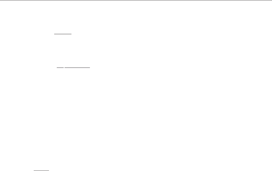
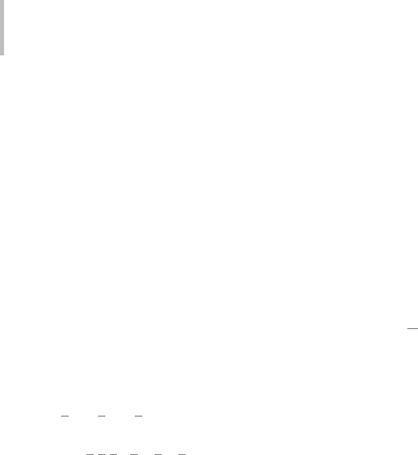
arranged as a star or as a triangle, see Figure 1.

Using Kirchhoff’s laws, the two situations in Figure 1

can be shown to be equivalent provided

¼ Z

þ Z

½1

=ðZ

þ Z

Þ½2

Here one has to take either [1] or [2] as second line

of the equation, depending on which direction the

transformation is to go. The star–triangle transfor-

mation thus defined is also known under other

names within the electric network theory literature

as wye–delta (Y  ), upsilon–delta (  ), or

tau–pi (T  ) transformation.

Spin Models

When Onsager wrote his monumental paper on the

Ising model published in 1944, he made a brief

remark on an obvious star–triangle transformation

relating the model on the honeycomb lattice with

the one on the triangular lattice. His details on this

were first presented in Wannier’s review article of

1945. However, the star–triangle transformati on

played a much more crucial role in Onsager’s

reasoning, as it is also intimately connected with

his elliptic function uniformizing parametrization.

Furthermore, it implies the commutation of

transfer matrices and spin-chain Hamiltonians.

Only in his Battelle lecture of 1970 did Onsager

explain how he used this remarkable observation in

his derivation of the formula for the spontaneous

magnetization which he had announced as a

conference remark in 1948 and of which the first

complete derivation had been publi shed by Yang in

1952 using a completely different method.

Many other applications and generalizations have

since appeared. Most generally, we can consider a

system whose state variables – also called spins – take

values from some suitable discrete or continuous sets.

The interactions between spins a and b are given in

termsofweightfactorsW

and W

,whichare

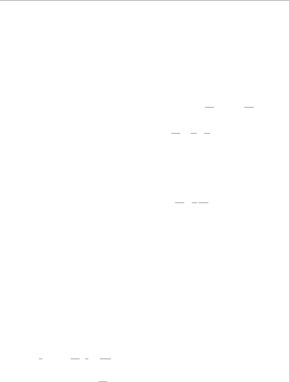
complex numbers in general, see Figure 2.One

quantity of special interest is the partition function –

sum of the product of all weight factors over all

allowed spin values. The integrability of the model is

expressed by the existence of spectral variables –

rapidities p, q, r, ... – that live on oriented lines, two

of which cross between a and b as indicated by the

dotted lines in Figure 2. Arrows from a to b are added

to keep track of the ordering of a and b in case the

weights are chiral (not symmetric).

In Onsager’s special choice of the Ising model the

spins take values a, b, c, ... = 1 and the weight

factors are the usual real positive Boltzmann weights

depending on the product ab = 1, uniformizing

variable p  q, and elliptic modulus k. In the integra-

ble chiral Potts model the weights depend on a  b

mod N,witha, b = 1, ..., N, whereas the rapidities p

and q are living in general on a higher-genus curve.

When the weights are asymmetric in the spins, there

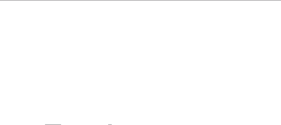
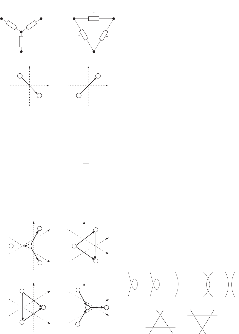
are two sets of star–triangle equations which can be

expressed both pictorially (Figure 3) and algebraically:

ðp; qÞW

ðq; rÞW

ðp; rÞ

¼ Rðp; q; rÞW

ðp; qÞW

ðq; rÞW

ðp; rÞ½3

Rðp; q; rÞW

ðp; qÞW

ðq; rÞW

ðp; rÞ

ðp; qÞW

ðq; rÞW

ðp; rÞ½4

Note that eqns [3] and [4] differ from each other by the

transposition of both spin variables in all six weight

factors. In general, there may also appear scalar factors

R(p, q, r)and

R(p, q, r), which can often be eliminated

by a suitable renormalization of the weights. If a, b,

and c take values in the same set, we can sum over

a = b = c, showing that R =

R in that case.

The Kennelly star–triangle equation [1], [2] can be

recovered as a special limit of a spin model where

the states are continuous variables.

Knot Theory and Braid Group

A seemingly totally different situ ation occurs in the

theory of knots, links, tangles, and braids. In 1926,

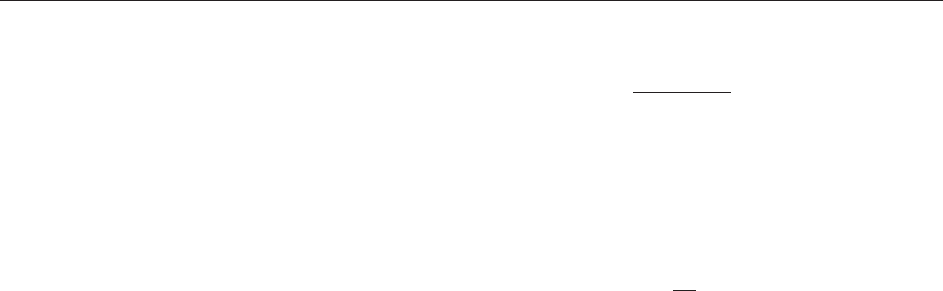
Reidemeister showed that only three types of moves

suffice to show the equivalence between two

different configurations, see Figure 4. Moves of

type I – removing simple loops – do not apply to

braids. Moves of type II, for which one strand crosses

twice over another strand, can be reformulated for

braids, namely that an overcrossing is the inverse of

an undercrossing. The Reidemeister move of type III

is a precursor of the more general Yang–Baxter

moves and can be represented also by the defining

relations of Artin’s braid group. Let R

i, iþ1

be the

operator representing the situation in which the

strand in position i crosses over the one in position

i þ 1. Then a braid can be represented by a product

of R

j, jþ1

’s and their inverses, provided

i;iþ1

iþ1;iþ2

i;iþ1

¼ R

iþ1;iþ2

i;iþ1

iþ1;iþ2

½5

and

½R

i;iþ1

; R

j;jþ1

¼0; if ji  jj2 ½6

and similar relations in which R

i, iþ1

and/or R

iþ1, iþ2

are replaced by their inverses.

Factorizable S-Matrices and Bethe Ansatz

In the early 1960s, Lieb and Liniger solved the one-

dimensional Bose gas with delta-function interaction

using the Bethe ansatz. Yang and McGuire then tried

to generalize this result to systems with internal

degrees of freedom and to fermions. This led to the

Figure 2 Spin model weights W

(p, q) and W

(p, q):

Figure 3 Star–triangle equation.

Figure 4 Reidemeister moves of types I, II, and III.

Figure 1 Star–triangle equation for impedances.

466 Yang–Baxter Equations

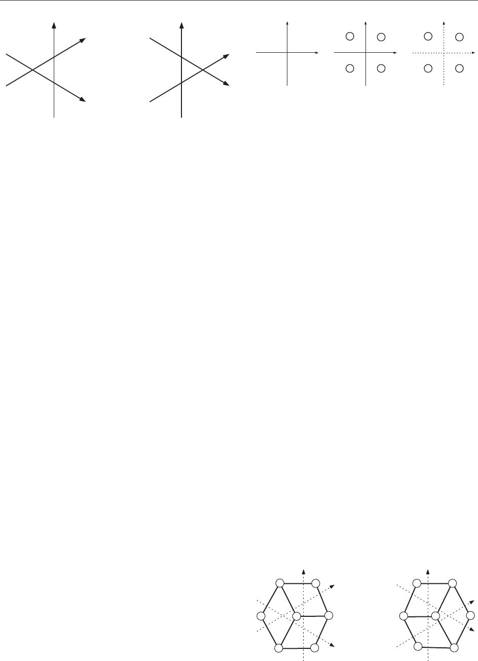
discovery of the condition for factorizable S-matrices

by McGuire in 1964, represented pictorially by

Figure 5, where the world lines of the particles are

given. Upon collisions the particles can only exchange

their rapidities p, q, r, so that there is no dispersion.

Also indicated are the internal degrees of freedom in

Greek letters. In other words, the three-body S-matrix

can be factorized in terms of two-body contributions

and the order of the collisions does not affect the

final outcome. McGuire also realized that this

condition is all one needs for the consistency of

factoring the n-body S-matrix in terms of two-body

S-matrices. The consistency condition is obviously

related to the Reidemeister move of type III in

Figure 4.

Yang su cceeded in solving the spin-1/2 fermionic

model using a nested Bethe ansatz, utilizing a

generalization of Artin’s braid relations [5] and [6],



i;iþ1

ðp  qÞ



iþ1;iþ2

ðp  rÞ



i;iþ1

ðq  rÞ



iþ1;iþ2

ðq  rÞ



i;iþ1

ðp  rÞ



iþ1;iþ2

ðp  qÞ½7

He submitted his findings in two short papers in

1967. The



R operators in eqn [7] – a notation

introduced later by the Leningrad school – depend

on differences of two momenta or two relativistic

rapidities. Sutherland solved the general spin case

using repeated nested Bethe ansa¨ tze, while Lieb and

Wu used Yang’s work to solve the one-dimensional

Hubbard model.

Vertex Models

Since Lieb’s solution of the ice model by a Bethe

ansatz, there have been many developments on

vertex models, in which the state variables live on

line segments and weight factors !





are assigned to

a vertex where four line segments with the four

states , , ,  on them meet, see Figure 6.

Baxter solved the eight-vertex model in 1971, using

a method based on commuting transfer matrices,

starting from a solution of what he then called the

generalized star–triangle equation, but what is now

commonly called the Yang–Baxter equation (YBE):













ðp; qÞ!







ðq; rÞ!







ðp; rÞ













ðp; qÞ!







ðq; rÞ!







ðp; rÞ½8

This equation is represented graphically in Figure 5.

From it one can also derive a sufficient condition for

the commutation of transfer matrices and spin-chain

Hamiltonians, generalizing the work of McCoy and

Wu, who had earlier initiated the search by showing

that the general six-vertex model transfer matrix

commutes with a Heisenberg spin-chain Hamilto-

nian. To be more precise, Baxter found that if





= 











for some choice of p and q, some spin-

chain Hamiltonians could be derived as logarithmic

derivatives of the transfer matrix.

Interaction-Round-a-Face Model

Baxter introduced another language, namely that of the

IRF or ‘ ‘interaction-round-a-face’ ’ model, which he

introduced in connection with his solution of the hard-

hexagon model. This formulation is convenient when

studying one-point functions using the corner-transfer-

matrix method. Now the integrability condition can be

represented graphically as in Figure 7 or algebraically as

ðp; qÞw

ðq; rÞw

ðp; rÞ

ðp; qÞw

ðq; rÞw

ðp; rÞ½9

The spins live on faces enclosed by rapidity lines and

the weights w

(p, q) are assigned as in Figure 6.

α′

α″

″

′

γ′

γ″

α″

α′

″

′

γ′

γ″

Figure 5 Vertex model YBE.

μμ

Figure 6 Vertex model weight !





(p, q), mixed model weight





(p, q) and IRF model weight w

(p, q).

a′

′

b′

′

b′

Figure 7 IRF model YBE.

Yang–Baxter Equations 467