Francoise J.-P., Naber G.L., Tsun T.S. (editors) Encyclopedia of Mathematical Physics
Подождите немного. Документ загружается.

Baxter discovered a new principle based on eqns [8]
and [9], which he called Z-invariance, as it expresses
an invariance of the partition function Z under moves
of rapidity lines. This also implies that typical one-
point functions are independent of the values of the
rapidities, while two-point functions can only depend
on the values of the rapidities of rapidity lines crossing
between the two spins considered. Many recent results
on correlation functions in integrable models depend
on this observation of Baxter.
IRF-Vertex Model
In Figure 6, we have also defined mixed IRF-vertex
model weights W
j
dc
ab
(p, q). (We could put further
state variables on the vertices, but then the natural
thing to do is to introduce new effective weights
summing over the states at each vertex.) With the
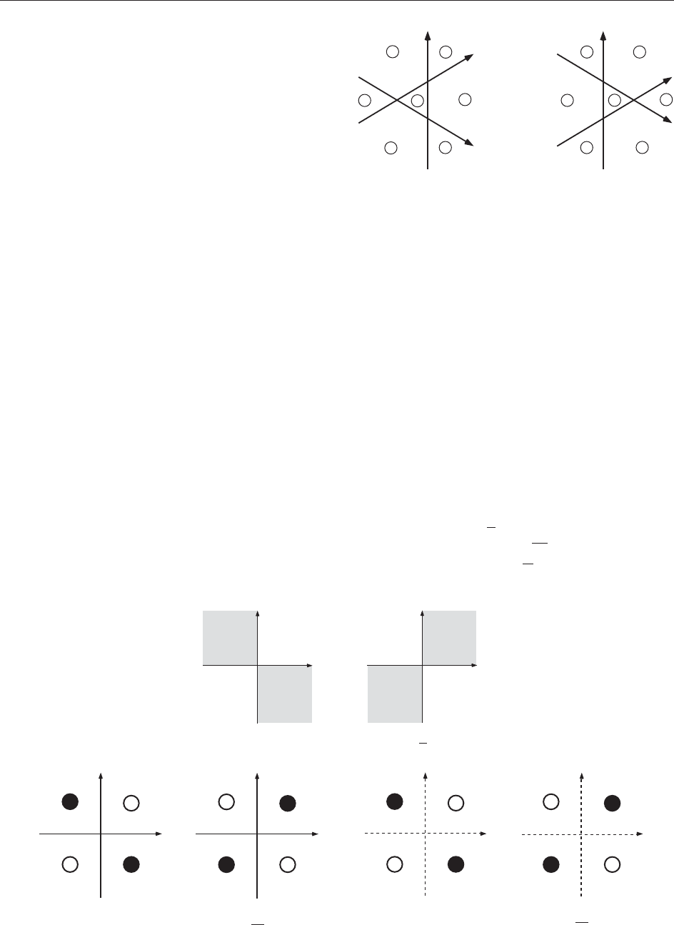
choice made a more general YBE can be represented
as in Figure 8,orby
X
00
X
00
X
00
X
d
W
00
00
j
a
0
d
cb
0
ðp; qÞ
W
0
0
00
00
j
a
0
b
dc
0
ðq; rÞW
00
0
00
j
dc
0
b
0
a
ðp; rÞ
¼
X
00
X
00
X
00
X
d
0
W
0
0
00
00
j
bc
0
d
0
a
ðp; qÞ
W
00
00
j
cd
0
b
0
a
ðq; rÞW
0
00
00
j
a
0
b
cd
0
ðp; rÞ½10
Quantum Inverse-Scattering Method
The Leningrad school of Faddeev incorporated the
methods of Baxter and Yang in their so-called
quantum inverse-scattering method (QISM), coining
the term quantum YBEs (QYBEs) for eqns [8].If
special limiting values of p and q can be found, say as
h ! 0, such that !
=
þ O(h), one can reduce
[8] to the classical Yang–Baxter equations (CYBEs) by
expanding up to the first nontrivial order in expansion
variable h. These determine the integrability of certain
models of classical mechanics by the inverse-scattering
method and the existence of Lax pairs.
Checkerboard generalizations
Star–triangle equations [3] and [4] imply that there are
further generalizations of the YBEs, namely those for
which the faces enclosed by the rapidity lines are
alternatingly colored blackandwhiteinacheckerboard
pattern. We can then introduce either vertex model
weights !
(p, q)and!
(p, q), or IRF-vertex model
weights W
j
dc
ab
(p, q)andW
j
dc
ab
(p, q), or IRF
model weights w
dc
ab
(p, q)andw
dc
ab
(p, q), see Figure 9.
a′
a
a
a′
d
bb
b′
b′
d
′
c
′ c ′
c
c
p
p
q
q
r
r
α
″
α′
α
α′
α
″
α
β
β
′′
β ′
β′
β
β
″
γ′
γ
″
γ
γ′
γ
″
γ
=
Figure 8 General YBE.
μ
μ
ααββ
λ
λ
p
p
q
q
ωω
μ
α
β
λ
p
q
b
d c
a
μ
αβ
λ
p
q
b
d c
a
p
q
b
d
c
a
p
q
b
d
c
a
W
W
w
w
Figure 9 Checkerboard versions of the weights.
468 Yang–Baxter Equations
The black faces are those where the spins of the
spin model with weights defined in Figure 2 live; the
white faces are to be considered empty in Figures 2
and 3 (or, equivalently, they can be assumed to host
trivial spins that take on only a single value).
Clearly, the IRF-ver tex model description contains
all the other versions.
Checkerboard Vertex Model
First we consider the checkerboard vertex model
with weights !
(p, q) and !
(p, q) as assigned in
Figure 9. The YBE [8] then generalizes to two sets of
equations:
X
00
X
00
X
00
!
00
00
ðp; qÞ!
0
0
00
00
ðq; rÞ!
00
0
00
ðp; rÞ
¼ Rðp; q; rÞ
X
00
X
00
X
00
!
0
0
00
00
ðp; q Þ
!
00
00
ðq; rÞ!
0
00
00
ðp; rÞ½11
Rðp;q;rÞ
X
00
X
00
X
00
!
00
00
ðp;qÞ!
0
0
00
00
ðq;rÞ!
00
0
00
ðp;rÞ
¼
X
00
X
00
X
00
!
0
0
00
00
ðp;qÞ!
00
00
ðq;rÞ!
0
00
00
ðp;rÞ½12
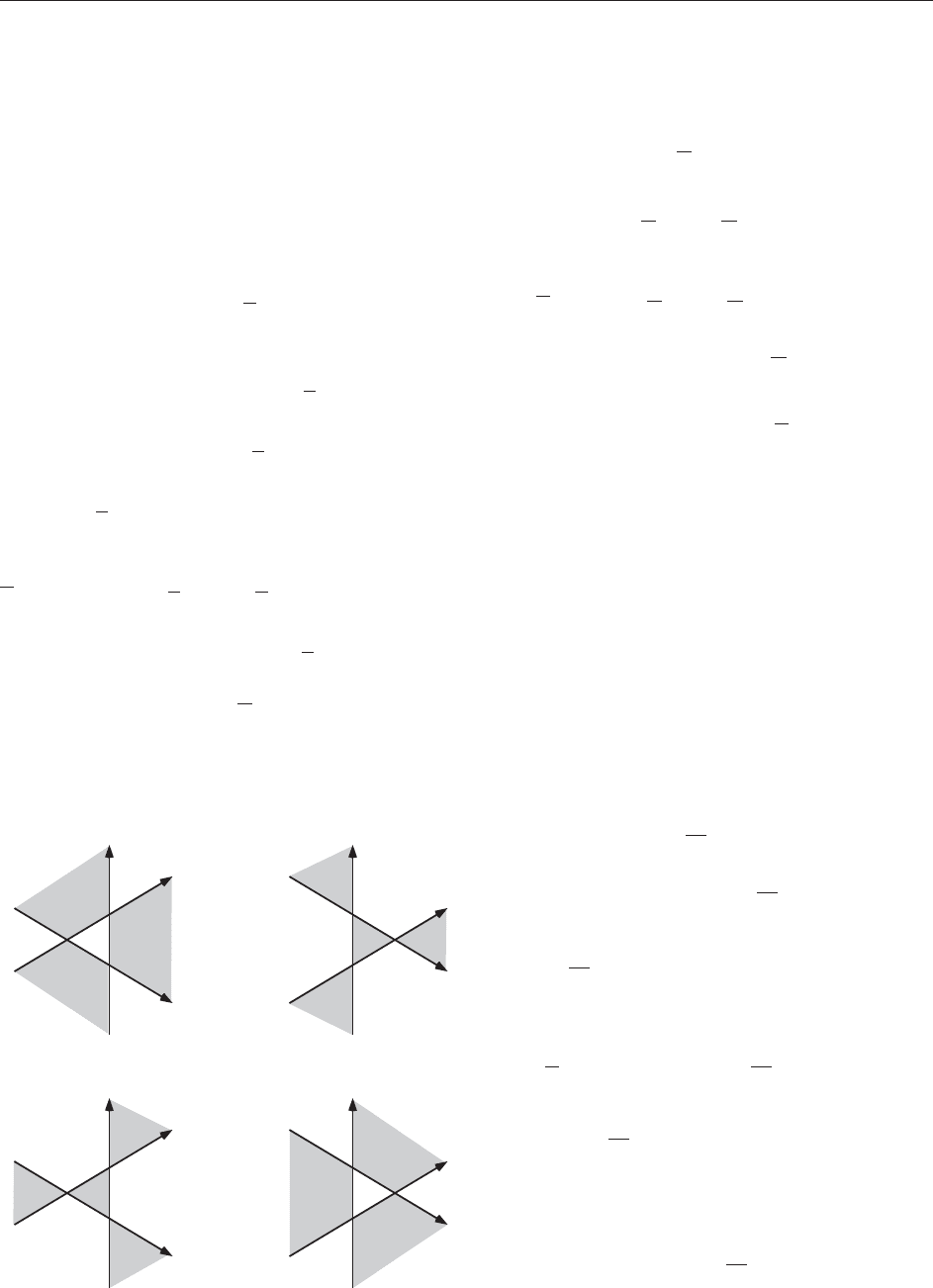
where scalar factors R and
R have been added as in
[3] and [4]. These equations are represented graphi-
cally by Figure 10.
Checkerboard IRF Model
The checkerboard IRF version of the YBE [8]
becomes
X
d
w
a
0
d
cb
0
ðp; qÞw
a
0
b
dc
0
ðq; rÞw
dc
0
b
0
a
ðp; rÞ
¼ Rðp; q; rÞ
X
d
0
w
bc
0
d
0
a
ðp; qÞw
cd
0
b
0
a
ðq; rÞw
a
0
b
cd
0
ðp; rÞ½13
Rðp; q; rÞ
X
d
w
a
0
d
cb
0
ðp; qÞw
a
0
b
dc
0
ðq; rÞw
dc
0
b
0
a
ðp; rÞ
¼
X
d
0
w
bc
0
d
0
a
ðp; qÞw
cd
0
b
0
a
ðq; rÞw
a
0
b
cd
0
ðp; rÞ½14
again with scalar factors R and
R added as in [3]
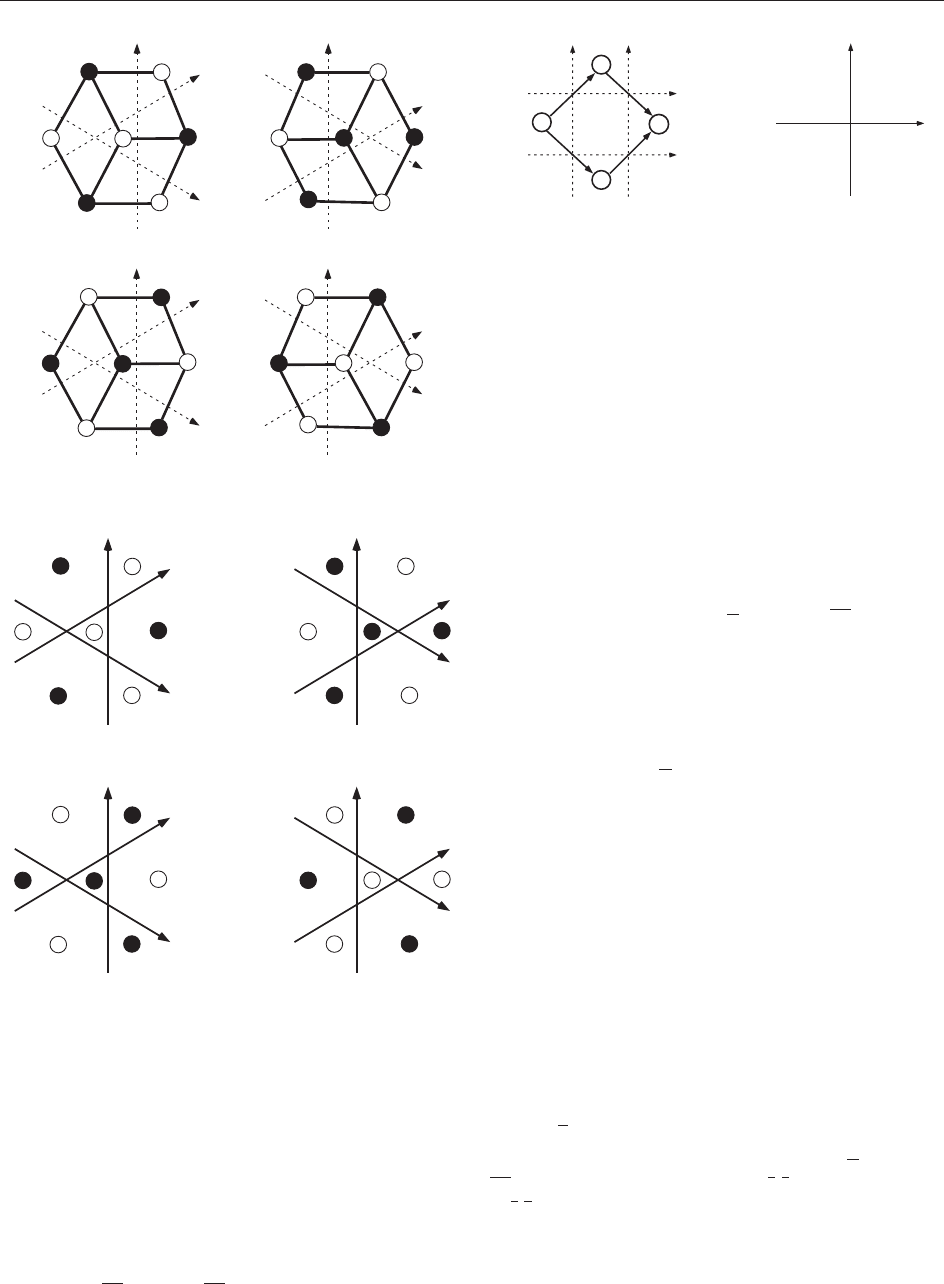
and [4]. These equations can now be represented
graphically as in Figure 11. Note that these
equations reduce to eqns [3] and [4] if the spins on
the white faces are allowed to take only one value,
which means that they can be ignored.
Checkerboard IRF-Vertex Model
Finally, the most general case is represented by the
checkerboard IRF-vertex model, with weights
defined in Figure 9. For this case the YBEs are
given by
X
00
X
00
X
00
X
d
W
00
00
j
a
0
d
cb
0
ðp; qÞ
W
0
0
00
00
j
a
0
b
dc
0
ðq; rÞW
00
0
00
j
dc
0
b
0
a
ðp; rÞ
¼ Rðp; q; rÞ
X
00
X
00
X
00
X
d
0
W
0
0
00
00
j
bc
0
d
0
a
ðp; qÞ
W
00
00
j
cd
0
b
0
a
ðq; rÞW
0
00
00
j
a
0
b
cd
0
ðp; rÞ½15
Rðp; q; rÞ
X
00
X
00
X
00
X
d
W
00
00
j
a
0
d
cb
0
ðp; qÞ
W
0
0
00
00
j
a
0
b
dc
0
ðq; rÞW
00
0
00
j
dc
0
b
0
a
ðp; rÞ
¼
X
00
X
00
X
00
X
d
0
W
0
0
00
00
j
bc
0
d
0
a
ðp; qÞ
W
00
00
j
cd
0
b
0
a
ðq; rÞW
0
00
00
j
a
0
b
cd
0
ðp; rÞ½16
with its graphical representation in Figure 12.
γ
α″
γ
′
α
β
β
′
α′
β ″
γ″
γ
α″
γ
′
α
β
β
′
α ′
β ″
γ″
γ
α″
γ
′
α
β
β
′
α′
β ″
γ″
γ
α″
γ
′
α
β
β
′
α′
β ″
γ″
p
p
p
p
q
q
q
q
r
r
r
r
=
=
Figure 10 Checkerboard vertex model YBE.
Yang–Baxter Equations 469
Formal Equivalence of Languages
The Square Weight
Combining four weights of a checke rboard model in
a square, as is done with four spin model weights
in Figure 13, we find a regular vertex model weight
with rapidities that are now pairs of the original
ones. This gives
W
ðp
1
; q
1
ÞW
ðp
1
; q
2
ÞW
ðp
2
; q
1
ÞW
ðp
2
; q
2
Þ
¼ !
ðp
1
; p
2
; q
1
; q
2
Þ½17
From any solution of [3] and [4] we can thus
construct a solution of YBE [8]. This has been used
by Bazhanov and Stroga nov to relate the integrable
chiral Potts model with a cyclic representation of the
six-vertex model.
Map to Checkerboard Vertex Model
The checkerboard IRF-vertex model formulation
contains all other versions mentioned above as
special cases. However, collecting the state variables
in triples, we can immediately translate it to a vertex
model version, writing
!
^
^
^
^
ðp; qÞ¼W
j
dc
ab
ðp; qÞ; !
^
^
^
^
ðp; q Þ¼W
j
dc
ab
ðp; qÞ
if
^
¼ðd;;cÞ;
^
¼ðb;;cÞ
^
¼ða;;dÞ;
^
¼ða;;bÞ
(
½18
!
^
^
^
^
ðp; qÞ¼!
^
^
^
^
ðp; qÞ¼0 otherwise ½19
In eqn [19], we have set all vertex model weights
zero that are inconsistent with IRF-vertex config-
urations. Clearly, the translation of IRF models and
spin models to vertex models can be done similarly.
Map to Spin Model
We can, furthermore, translate each vertex model
with weights assigned as in Figures 6 or 9 into a spin
model with weights as in Figure 2 by defining
suitable spins in the black faces, after checkerboard
coloring. Each spin is then defined to be the ordered
set of states on the line segments of the vertex
model,
a = (
1
,
2
, ...), ordering the line segments
counterclockwise starting at, say, 12 o’clock. We
can then identify !
(p, q) = W
a, b
(p, q), !
(p, q) =
W
a, b
(p, q). This is surely not very economical, as
many of the weights will be equal, but it helps show
that all different versions of the checkerboard YBE
are formally equivalent.
Hence, we shall only use the vertex model
language in the following. It is fairly straightforward
to convert to the other formulations.
γ
α′′
γ′
α
β
β′
α′
β′′
γ′′
γ
α″
γ′
α
β
β′
α′
β″
γ″
γ
α
″
γ′
α
β
β′
α′
β″
γ″
γ
α″
γ′
α
β
β′
α
′
β″
γ″
a′
a′
a
a
a
a
a′
a′
b
b
b
b
′
b′
b
b′
b′
c
c
′
c
c′
c ′
c
c′
c
d
d
′
d ′
d
p
p
p
p
q
q
q
q
r
r
rr
=
=
Figure 12 Checkerboard YBE.
a
a
a
a
a′ a′
a′
a′
d
d
′
d
′d
b
b
bb
b′
b′
b
′
b′
c
c
′
c
′
c
c
c
′
c
′
c
p
p
p
p
q
q
q
q
r
r
r
r
=
=
Figure 11 Checkerboard IRF model YBE.
α
λ
β
μ
α
λ
β
μ
p
2
p
1
q
1
q
2
=
(p
1
,p
2
)
(q
1,
q
2
)
Figure 13 Square weight as vertex weight.
470 Yang–Baxter Equations
An sl(mjn) Example
One fundamental example is a Q-state model for
which the rapidities have 2Q þ 1 components,
p = (p
Q
, ..., p
Q
), q = (q
Q
, ..., q
Q
), etc., and the
states on the line segments are arranged in strings
of continuing conserved color. The vertex weights,
for , , , ¼1, ..., Q, are given by
!
ðp; qÞ¼!
0
ðp
0
; q
0
Þ
p
þ
q
q
þ
p
½20
with ( 6¼ )
!
0
ðp
0
; q
0
Þ¼Nsinh½ þ "
ðp
0
q
0
Þ
!
0
ðp
0
; q
0
Þ¼NG
sinhðp
0
q
0
Þ
!
0
ðp
0
; q
0
Þ¼Ne
ðp
0
q
0
ÞsignðÞ
sinh
!
0
ðp
0
; q
0
Þ¼0; otherwise
½21
where N is an arbitrary overall normalization factor
and is a constant. Furthermore, "
= 1 for
= 1, ..., Q, where m of them equal þ1 and n of
them equal 1. The G
’s are constants satisfying
G
= 1=G
, which freedom is allowed because the
number of - crossings minus the number of -
crossings is fixed by the states on the boundary only,
that is, the choice of ,
0
, ,
0
, ,
0
in YBE [8] and
Figure 5.
The solution [20], [21] has many applications.
The case m = 0, n = 2 leads to the general six-vertex
model; the m = 0, n = n case produces the funda-
mental intertwiner of affine quantum group U
q
b
sl(n),
whereas the case m = 2, n = 1 corresponds to the
supersymmetric one-dimensional t–J model.
Operator Formulations
The R-Matrix
For a problem with N rapidity lines, carrying
rapidities p
1
, ..., p
N
, we can introduce a set of
matrices R
ij
(p
i
, p
j
), for 14i < j4N, with elements
R
ij
ðp
i
; p
j
Þ
1
...
N
1
...
N
¼ !
j
i
i
j
ðp
i
; p
j
Þ
Y
k6¼i; j
k
k
½22
In terms of these, the YBE [8] can be rewritten in
matrix form as
R
jk
ðp
j
; p
k
ÞR
ik
ðp
i
; p
k
ÞR
ij
ðp
i
; p
j
Þ
¼ R
ij
ðp
i
; p
j
ÞR
ik
ðp
i
; p
k
ÞR
jk
ðp
j
; p
k
Þ
½23
where 14i < j < k4N.
The
ˇ
R-Matrix
If we transpose the indices
i
and
j
in eqn [22],
we can define a set of matrices
ˇ
R
i, iþ1
(p, q) with
elements
ˇ
R
i; iþ1
ðp; qÞ
1
...
N
1
...
N
¼ !
i
;
iþ1
i
;
iþ1
ðp; qÞ
Y
k6¼i; iþ1
k
k
½24
Using these, the YBE [8] can be rewritten in matrix
form as
ˇ
R
i; iþ1
ðq; rÞ
ˇ
R
iþ1; iþ2
ðp; rÞ
ˇ
R
i; iþ1
ðp; q Þ
¼
ˇ
R
iþ1; iþ2
ðp; qÞ
ˇ
R
i; iþ1
ðp; rÞ
ˇ
R
iþ1; iþ2
ðq; rÞ½25
and
½
ˇ
R
i; iþ1
ðp; qÞ;
ˇ
R
j; jþ1
ðr; sÞ ¼ 0; if ji jj52 ½26
In this formulation, it is clear that many solutions
can be found ‘‘Baxterizing’’ Temperley–Lieb and
Iwahori–Hecke algebras.
Classical YBEs
If we expand
R
ij
ðp
i
; p
j
Þ¼1 þ hX
ij
ðp
i
; p
j
ÞþOðh
2
Þ½27
in [23], we get in second order in h the classical YBE
(CYBE) as the vanishing of a sum of three commu-
tators, that is,
½X
ij
ðp
i
; p
j
Þ; X
ik
ðp
i
; p
k
Þ þ ½X
ij
ðp
i
; p
j
Þ; X
jk
ðp
j
; p
k
Þ
þ½X
ik
ðp
i
; p
k
Þ; X
jk
ðp
j
; p
k
Þ ¼ 0 ½28
introduced by Belavin and Drinfel’d, where X
ij
is
called the classical r-matrix.
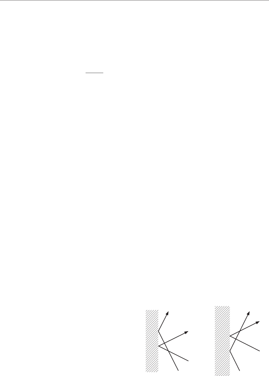
Reflection YBEs
Cherednik and Sklyanin found a condition deter-
mining the solvability of systems with boundaries,
the reflection YBEs (RYBEs), see Figure 14. Upon
q
–
p
–
p
q
q
–
p
–
p
q
=
Figure 14 Reflection YBE.
Yang–Baxter Equations 471
collisions with a left or right wall the rapidity
variable changes from p to p and back. In most
examples, in which the rapidities are difference
variables such that R(p, q) = R(p q), one also has
p = p,with some constant. The corresponding
left boundary weights are K
(p, p) satisf ying
ˇ
K
1
ðq; qÞ
ˇ
R
12
ðp; qÞ
ˇ
K
1
ðp; pÞ
ˇ
R
12
ðq; pÞ
¼
ˇ
R
12
ðp; qÞ
ˇ
K
1
ðp; pÞ
ˇ
R
12
ðq; pÞ
ˇ
K
1
ðq; qÞ½29
with
ˇ
K
1
(p, p) de fined by a direct product as in [24]
appending unit matrices for positions i52, and a
similar equation must hold for the right boundary.
Most work has been done for vertex models, while
Pearce and co-workers wrote several papers on the
IRF-model version.
Higher-Dimensional Generalizations
In 1980 Zamolodchikov introduced a three-
dimensional generalization of the YBE, the so-called
tetrahedron equations (TEs), and he found a special
solution. Baxter then succeeded in proving that
this solution satisfies all TEs. Baxter and Bazhanov
showed in 1992 that this solution can be seen as
a special case of the sl(1) chiral Potts model.
Several authors found furth er generalizations more
recently.
Inversion Relations
When !
(p, p) /
, that is, the weight decouples
when the two rapidities are equal, one can derive the
local inverse relati on depicted in Figure 15, which is
a generalization of the Reidemeister move of type II
in Figure 4. It is easily shown that C(q, p) = C(p, q).
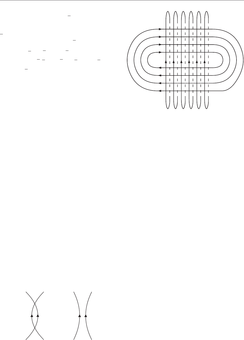
This local relatio n implies also a global inversion
relation which can be found in many ways. The
following heuristic way is the easiest: consider the
situation in Figure 16, with N closed p-rapidity lines
and M closed q-rapidity lines. For M and N large,
we may expect the partition function of Figure 16
to factor asymptotically in top- and bottom-half
contributions. If each line segment carries a state
variable that can assume Q values, then the total
partition function factors by repeated application of
the relation in Figure 15 into the contribution of
M þ N circles. Therefore,
Z ¼ Q
MþN
Cðp; qÞ
MN
Z
M; N
ðp; q ÞZ
N; M
ðq; pÞ½30
Taking the thermodynamic limit,
zðp; qÞ lim
M; N!1
Z
M; N
ðp; q Þ
1=MN
½31
one finds
zðp; qÞzðq; pÞ¼Cðq; pÞ½32
In many models, eqn [32], supplemented with some
suitable symmetry and analyticity conditions, can be
used to calculate the free energy per site.
See also: Affine Quantum Groups; Bethe Ansatz;
Classical r-matrices, Lie Bialgebras, and Poisson Lie
Groups; Eight Vertex and Hard Hexagon Models; Hopf
Algebras and q-Deformation Quantum Groups;
Integrability and Quantum Field Theory; Integrable
Discrete Systems; Integrable Systems: Overview; The
Jones Polynomial; Knot Invariants and Quantum Gravity;
Knot Theory and Physics; Sine-Gordon Equation;
Topological Knot Theory and Macroscopic Physics;
Two-Dimensional Ising Model; von Neumann Algebras:
Subfactor Theory.
Further Reading
Au-Yang H and Perk JHH (1989) Onsager’s star-triangle
equation: master key to integrability. Advanced Studies in
Pure Mathematics 19: 57–94.
Baxter RJ (1982) Exactly Solved Models in Statistical Mechanics.
London: Academic Press.
qp pq
C(p,q)
=
Figure 15 Local inversion relation.
p
p
p
p
qqqqqq
p
p
p
p
Figure 16 Heuristic derivation of inversion relation.
472 Yang–Baxter Equations

Behrend RE, Pearce PA, and O’Brien DL (1996) Interaction-
round-a-face models with fixed boundary conditions: the ABF
fusion hierarchy. Journal of Statistical Physics 84: 1–48.
Gaudin M (1983) La Fonction d’Onde de Bethe. Paris: Masson.
Jimbo M (ed.) (1987) Yang–Baxter Equation in Integrable
Systems. Singapore: World Scientific.
Kennelly AE (1899) The equivalence of triangles and three-
pointed stars in conducting networks. Electrical World and
Engineer 34: 413–414.
Korepin VE, Bogoliubov NM, and Izergin AG (1993) Quantum
Inverse Scattering Method and Correlation Functions.
Cambridge: Cambridge University Press.
Kulish PP and Sklyanin EK (1981) Quantum spectral transform
method. Recent developments. In: Hietarinta J and
Montonen C (eds.) Integrable Quantum Field Theories,
Lecture Notes in Physics, vol. 151, pp. 61–119. Berlin:
Springer.
Lieb EH and Wu FY (1972) Two-dimensional ferroelectric
models. In: Domb C and Green MS (eds.) Phase Transitions
and Critical Phenomena, vol. 1, pp. 331–490. London:
Academic Press.
Onsager L (1971) The Ising model in two dimensions. In: Mills
RE, Ascher E, and Jaffee RI (eds.) Critical Phenomena in
Alloys, Magnets and Superconductors, pp. xix–xxiv, 3–12.
New York: McGraw-Hill.
Perk JHH (1989) Star-triangle equations, quantum Lax pairs, and
higher genus curves. Proceedings of Symposia in Pure
Mathematics 49(1): 341–354.
Perk JHH and Schultz CL (1981) New families of commuting
transfer matrices in q-state vertex models. Physics Letters A
84: 407–410.
Perk JHH and Wu FY (1986) Graphical approach to the
nonintersecting string model: star-triangle equation, inversion
relation, and exact solution. Physica A 138: 100–124.
Reidemeister K (1926a) Knoten und Gruppen. Abhandlungen aus
dem Mathematischen Seminar der Hamburgischen Universita¨t
5: 7–23.
Reidemeister K (1926b) Elementare Begru¨ ndung der Knotenthe-
orie. Abhandlungen aus dem Mathematischen Seminar der
Hamburgischen Universita¨t 5: 24–32.
Yang CN (1967) Some exact results for the many-body problem
in one dimension with repulsive delta-function interaction.
Physical Review Letters 19: 1312–1314.
Yang CN (1968) S-matrix for the one-dimensional N-body
problem with repulsive or attractive -function interaction.
Physical Review 167: 1920–1923.
Yang–Baxter Equations 473