Francoise J.-P., Naber G.L., Tsun T.S. (editors) Encyclopedia of Mathematical Physics

Подождите немного. Документ загружается.

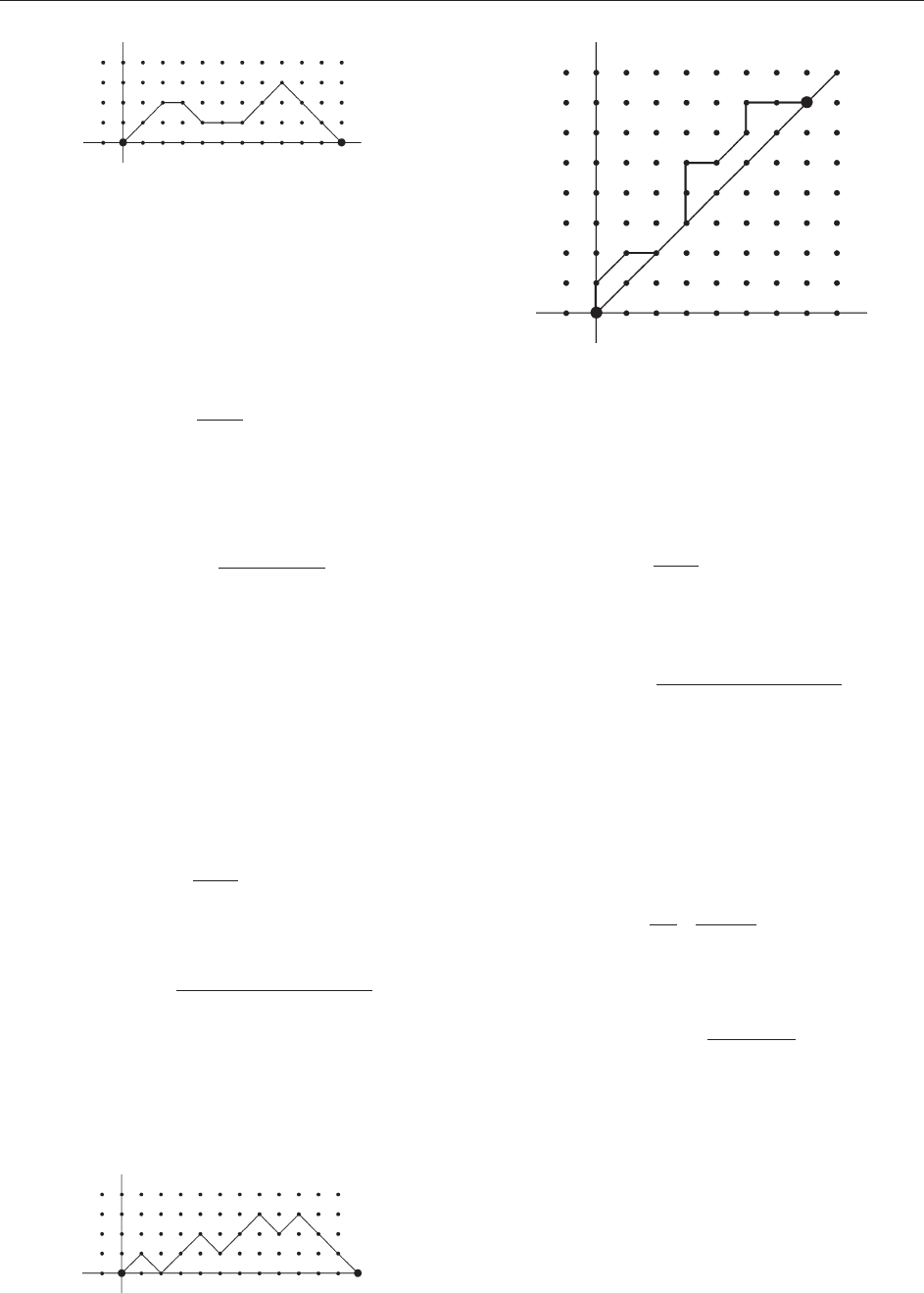
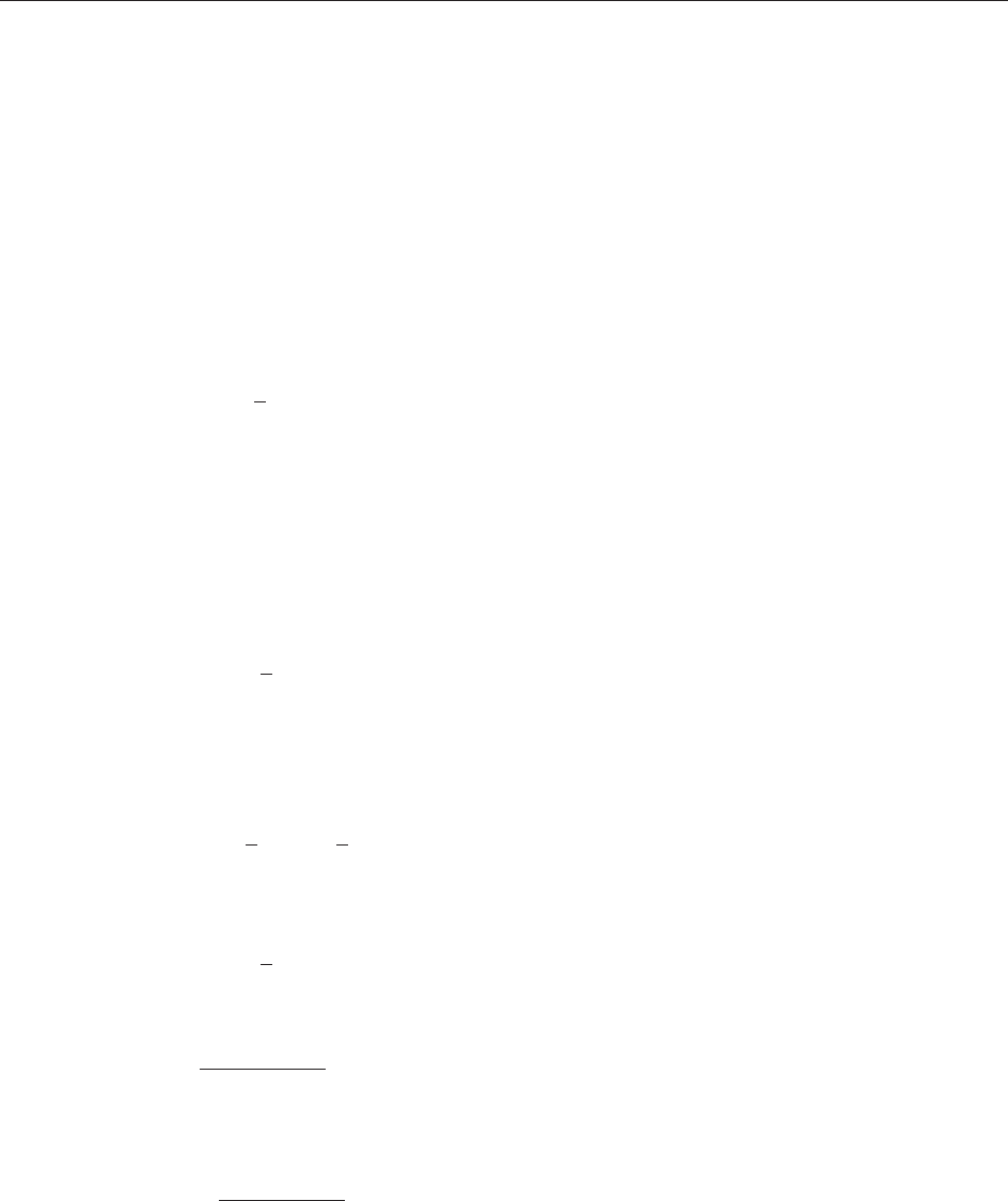
A Dyck path is a lattice path in the integer

plane Z

consisting of up-steps (1, 1) and down-steps

(1, 1), which starts at the origin, never passes below

the x-axis, and ends on the x-axis. See Figure 3 for an

example.

The number of Dyck paths of length 2n is the

Catalan number

n þ 1



The generating function (see the next section for an

introductiontothetheoryofgeneratingfunctions)

for these numbers is

n¼0

1 

ﬃﬃﬃﬃﬃﬃﬃﬃﬃﬃﬃﬃﬃﬃ

1  4x

½1

The reader is referred to exercise 6.19 in Stanley

(1999) for countless occurrences of the Catalan

numbers.

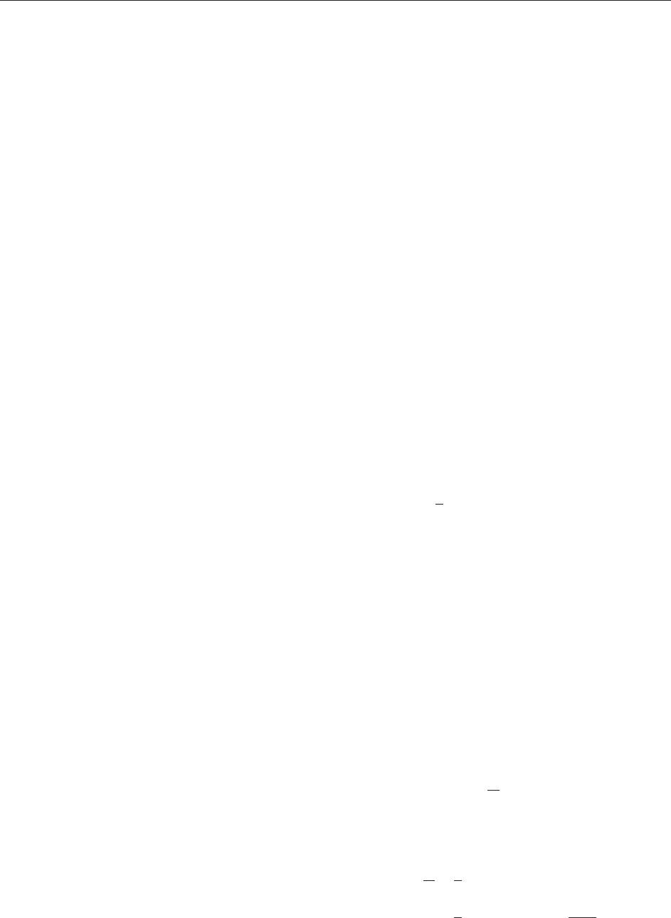
A Motzkin path is a lattice path in the integer

plane Z

consisting of up-steps (1, 1), level steps

(1, 0), and down-steps (1,1), which starts at the

origin, never passes below the x-axis, and ends on

the x-axis. The path in Figure 2 is in fact a Motzkin

path. The number of Motzkin paths of length n is

the Motzkin number

k0

k þ 1





The generating function for these numbers is

n¼0

1  x 

ﬃﬃﬃﬃﬃﬃﬃﬃﬃﬃﬃﬃﬃﬃﬃﬃﬃﬃﬃﬃﬃﬃﬃﬃﬃﬃﬃﬃ

1  2x  3x

½2

The reader is referred to exercise 6.38 in Stanley (1999)

for numerous occurrences of the Motzkin numbers.

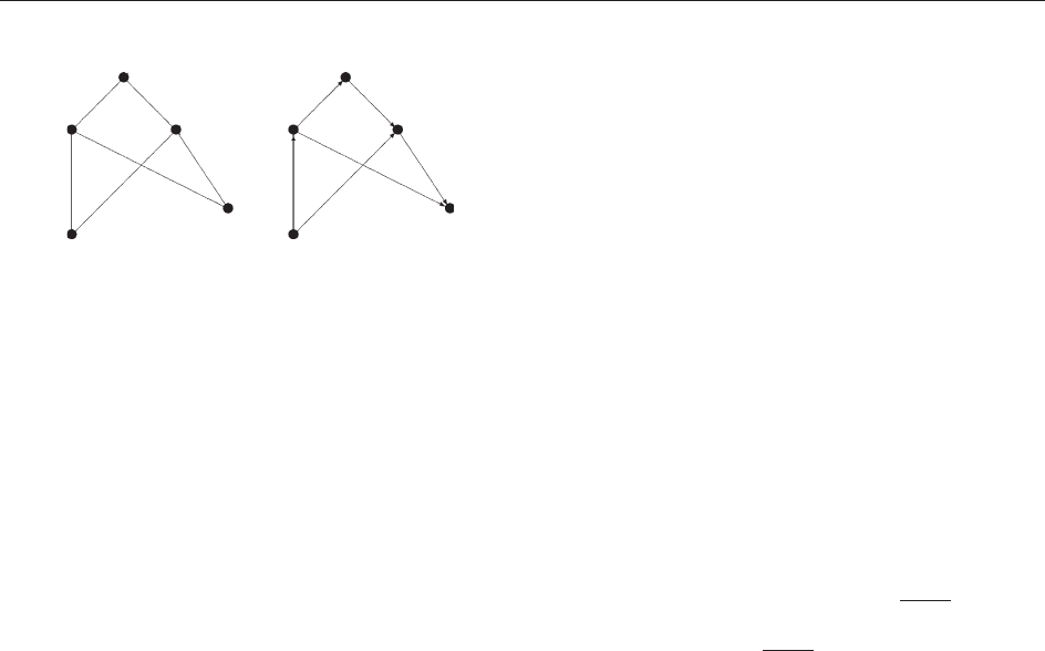
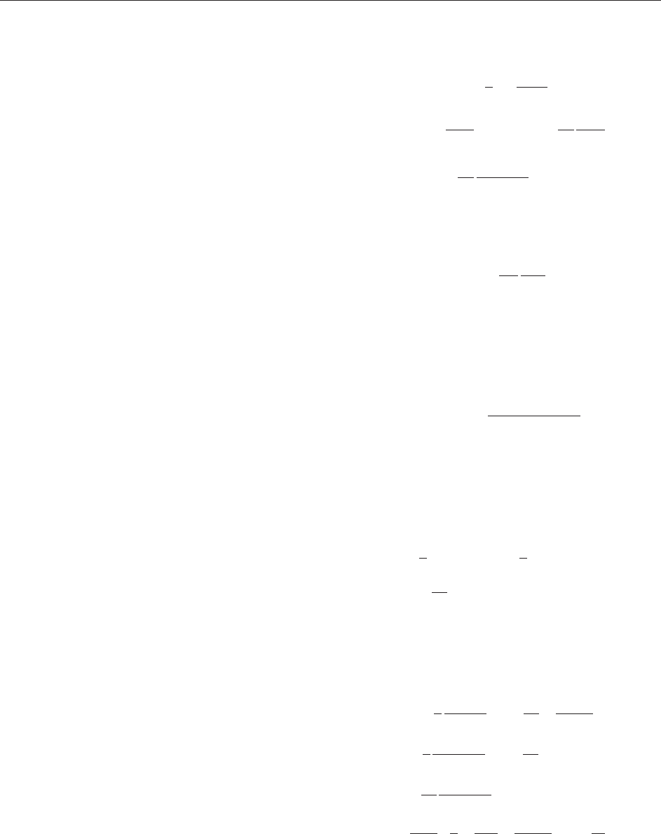
A Schro¨ der path is a lattice path in the integer

plane Z

consisting of horizontal steps (1, 0) and

vertical steps (0, 1), which starts at the origin, never

passes below the diagonal x = y, and ends on the

diagonal x = y. See Figure 4 for an example.

The number of Schro¨ der paths of length n is the

(large) Schro¨ der number

k0

k þ 1



n þ k



The generating function for these numbers is

n¼0

1  x 

ﬃﬃﬃﬃﬃﬃﬃﬃﬃﬃﬃﬃﬃﬃﬃﬃﬃﬃﬃﬃﬃﬃﬃﬃﬃ

1  6x þ x

½3

The reader is referred to exercise 6.39 in Stanley

(1999) for numerous occurrences of the Schro¨ der

numbers.

There is another famous sequence of numbers

which we did not touch yet, the Fibonacci numbers

. They are given by

ﬃﬃﬃ

1 þ

ﬃﬃﬃ

nþ1

with generating function

n¼0

1  x  x

½4

They also occur in numerous places. For example,

the number F

counts all paths on the integers Z

from 0 to n with steps (1, 0) and (2, 0).

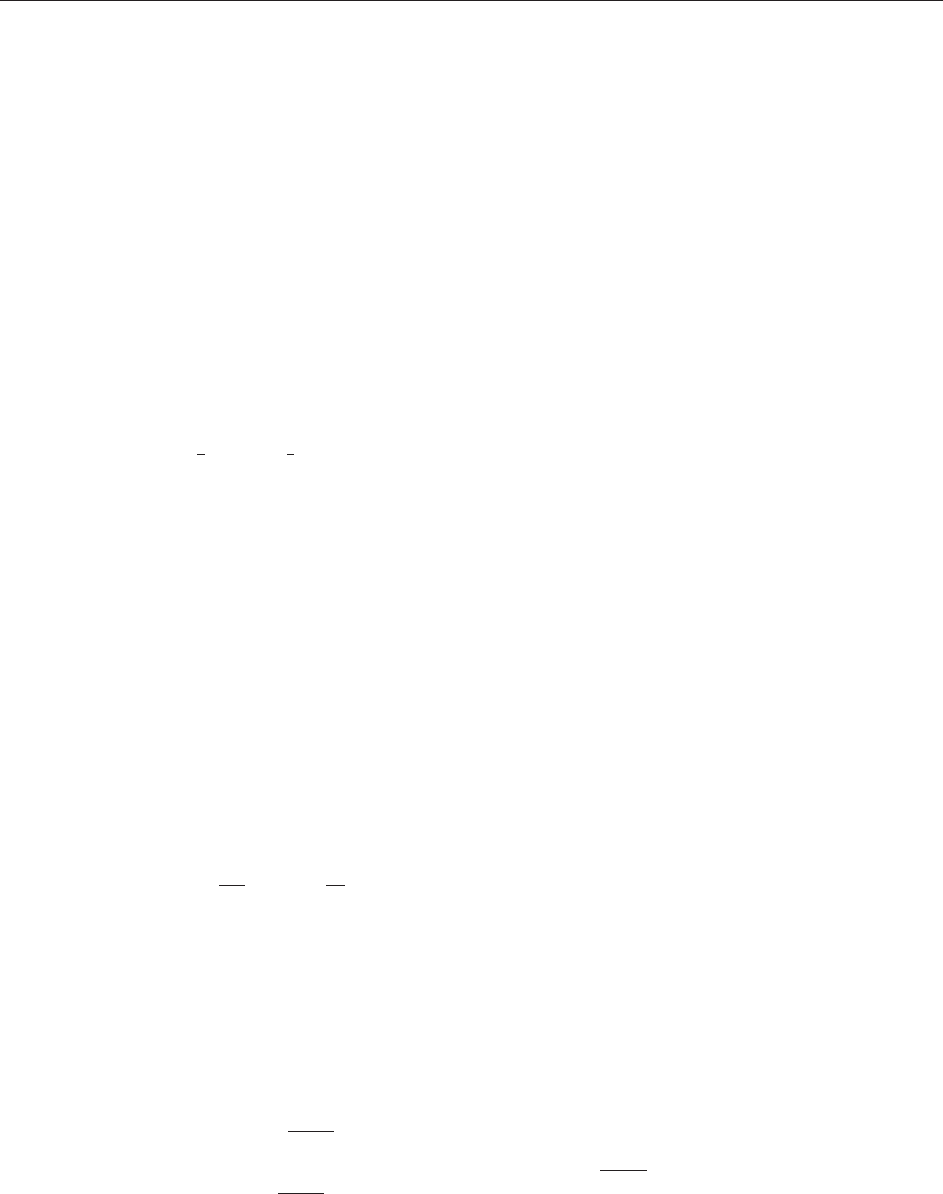
An undirected graph G consists of vertices and

edges. An edge is a two-element subset of the

vertices, which, however, is thought of as a line or

curve connecting the two vertices. See Figure 5a

for an example. The usual notation for a graph G

is G = (V, E), where V is the set of vertices and E

is the set of edges of G.Agraphisplanarifitis

Figure 2 A Motzkin path.

Figure 3 A Dyck path.

Figure 4 A Schro

der path.

Combinatorics: Overview 555

embedded in the plane (sphere) in such a way that

the curves which mark the edges do not intersect

in their interiors. There can be several different

ways to embed the same graph in the plane (or in

another surface). When we speak of a planar

graph then we assume the graph already to be

embedded in a given way. For example, the graph

in Figure 5 is not a planar graph, by its drawing.

However, there is a different embedding which is

planar (namely, all embeddings which put the

vertex v

above the vertex v

and leave the other

vertices as they are). A tree is a graph without any

cycles.

A directed graph (or digraph) G consists of

vertices and arcs (which are sometimes also called

directed edges). An arc is a pair of vertices, which,

however, is thought of an arrow pointing from the

first vertex of the pair to the second. See Figure 5b

for an example. The usual notation for a directed

graph G is again G = (V, E), where V is the set of

vertices and E is the set of arcs of G. All other

notions explained for undirected graphs have analo-

gous meanings for directed graphs.

Graphs can be labeled, in which case each vertex

is assigned a label, or unlabeled. The (undirected)

graph in Figure 5a is labeled, whereas the (directed)

graph in Figure 5b is unlabeled.

Generating Functions

Generating functions are the very basic tools of

enumeration. For introductions to this technique,

from different points of view, the reader is referred

to Bergeron et al. (1998), Flajolet and Sedgewick

(chapter1inthereferencelistedin‘‘Furtherread-

ing’’section),andStanley(1998,chapter1;1999,

chapter 4).

Let A be a set of (unlabeled) objects. Each object

a in A has a certain size, jaj, which is a non-negative

integer. Let us also assume that there is only a finite

number of objects from A of a given size. Let a

the number of objects from A of size n. The

(ordinary) generating function for A is the formal

power series

ðxÞ¼

a2A

jaj

n¼0

(‘‘formal’’ means that x is just an indeterminate, not

a real or complex number. One can compute with

formal power series in the same way as with analytic

series, only that convergence issues do not arise,

respectively that ‘‘convergence’’ has a different

meaning; cf. Stanley (1998, section 1.1)) Typical

examples are Sets (the collection containing all

‘‘unlabeled sets,’’ that is, all objects of the form

{•, •, ..., •}, including the empty set, where the size

of {•, •, ..., •} is the number of •’s), Sequences

(the collection containing all ‘‘unlabeled sequences,’’

that is, all objects of the form (•, •, ..., •), including

the empty sequence), Cycles (unlabeled cycles),

with respective generating function

Sets

ðxÞ¼F

Sequences

ðxÞ¼

1  x

Cycles

ðxÞ¼

1  x

½5

or Trees (unlabeled trees).

If A and B are two sets of objects, one can define

several other sets of objects using them. The union

of A and B, written A[B, has as a groundset the

disjoint union of A and B, and the size of an element

from A is its size in A, while the size of an element

from B is its size in B.Wehave

A[B

ðxÞ¼F

ðxÞþF

ðxÞ½6

The product of A and B, written AB, has as a

groundset the set of pairs AB, and the size of an

element (a, b) from ABis the sum of the sizes of a

(in A) and of b (in B). We have

AB

ðxÞ¼F

ðxÞF

ðxÞ½7

The substitution of two sets A and B of objects

can only be defined in certain circumstances, and

only in certain more restrictive circumstances the

generating function for the substitution can be

computed by substituting the generating functions

for A and B. Let us assume that any object a from

A of size n, by its structure, has n atoms (nodes). For

example, if A is a certain set of trees, where the size

of a tree is the number of leaves in the tree, then we

may take, as the atoms, the leaves of the tree. In this

situation, the substitution of B in A, denoted by

A(B), is the set of objects which arises by replacing

the atoms of objects from A by objects from B in all

possible ways. The size of an object from A(B) is the

sum of the sizes of the objects from B that it

(a) (b)

Figure 5 (a) An undirected graph. (b) A directed graph.

556 Combinatorics: Overview

contains. In order that A(B) contains only a finite

number of objects of a given size, we must assume

that B contains no elements of size 0. If, in addition,

the atoms of any element a from A inherit an order

(e.g., if A is a set of binary trees, then the leaves of a

binary tree are ordered in a natural way from ‘‘left’’

to ‘‘right’’), then we have

AðBÞ

ðxÞ¼F

ðF

ðxÞÞ ½ 8

However, this equation is not true in general. The

general formula comes out of Redfield–Po´lya theory

(see [21] and [24]) and requires the notion of cycle

index series. For example, if B is the set of connected

(unlabeled) graphs, A is Sets, so that A(B) is the

set of all (connected and disconnected) graphs, then

[8] is not true, but what is true is

SetsðBÞ

¼ exp F

ðxÞþ

ðx

Þþ

ðx

Þþ



½9

This holds, in fact, for any set B of unlabeled objects.

(This is seen by combining [24], [17], and [21].)

Next we deal with the enumeration of labeled

objects. Let A be a set of labeled objects, again, each

object a with a certain size jaj which is a non-

negative integer. ‘‘Labeled’’ means that each object

of size n, by its structure, comes with n atoms

(nodes) which are labeled 1, 2, ..., n. For example,

A may be the set of all labeled graphs, where the

size of a graph is the number of its vertices, and

where the vertices are labeled 1, 2, ..., n. Again, we

assume that there is only a finite number of objects

from A of a given size. Let a

be the number of

objects from A of size n. The exponential generating

function for A is the formal power series

ðxÞ¼

a2A

jaj

jaj!

n¼0

Typical examples are Sets (the collection containing

all ‘‘labeled sets,’’ that is all objects of the form

{1, 2, ..., n}, including the empty set), Permuta-

tions, Cycles (labeled cycles), with respective

generating functions

Sets

ðxÞ¼expðxÞ½10

Permutations

ðxÞ¼

1  x

½11

Cycles

ðxÞ¼log

1  x

½12

or Trees (labeled trees). The explicit form of the

generating function for Trees is discussed in the

section‘‘Solvingequationsforgeneratingfunctions:

theLagrangeinversionformulaandthekernel

method.’’

If A and B are two sets of objects, one defines

again several other sets of objects using them. The

union of A and B, written A[B, has as a groundset

the disjoint union of A and B, and the size of an

element from A is its size in A, while the size of an

element from B is its size in B. We have

A[B

ðxÞ¼E

ðxÞþE

ðxÞ½13

To define the product of A and B, written AB,

we cannot simply take AB as a groundset, we

must also say something about the labeling of the

objects. So, as a groundset we take all pairs (a, b)

with a 2A and b 2B, but labeled in all possible

ways by 1, 2, ..., ja jþjbj such that the order of

labels assigned to a respects the original order of

labels of a, and the same for b. The size of such an

element (a,b) is again the sum of the sizes of a (in A)

and of b (in B). We have

AB

ðxÞ¼E

ðxÞE

ðxÞ½14

Since, in the labeled world, objects come automati-

cally with atoms, the substitution of two sets A and

B of objects can now always be defined. The

substitution of B in A, denoted by A(B), is the set

of objects which arises by replacing the atoms of

objects from A by objects from B in all possible

ways, and labeling the substituted objects in all

possible ways by 1, 2, ...,

jbj (the sum being

over the objects from B which were put in the places

of the atoms) that are consistent with the original

labelings of the objects from B. The size of an object

from A(B) is the sum of the sizes of the objects from

B that it contains. In order that A(B) contains only a

finite number of objects of a given size, we must

assume that B contains no elements of size 0. Then

we have

AðBÞ

ðxÞ¼E

ðE

ðxÞÞ ½15

An example of a composition is

Permutations ¼ SetsðCyclesÞ

Thus, from [15] we have

Permutations

ðxÞ¼E

Sets

ðE

Cycles

ðxÞÞ

corresponding to the identity

1  x

¼ exp log 1=ð1  xÞðÞ

Another manifestation of the composition rule is, for

example, the fact (which is sometimes called the

‘‘exponential principle’’) that, if one takes the log of

the partition function for some maps, the result is

the partition function for the connected maps among

them.

Combinatorics: Overview 557

All of the above can be generalized to a weighted

setting. Namely, if A is a set of objects (labeled or

unlabeled), and if w : A!R is a weight function

from A into some ring R, then all of the above

remains true, if we replace the definitions of F

(x)

and E

(x) above by the weighted sums

ðxÞ¼

a2A

wðaÞx

jaj

and

ðxÞ¼

a2A

wðaÞ

jaj

jaj!

respectively, if in the definition of the union of A

and B we define the weight of an object to be its

weight in A, respectively B, if in the definition of the

product of A and B we define the weight of an

object (a, b) to be the product of the weights of a

and b, and if in the definition of the substitution we

define the weight of an object in A(B) as the product

of the weights of the objects from B that were put in

place of the atoms.

Redfield–Po´ lya Theory of Colored

Enumeration

The natural and uniform environment for the

separate treatment of generating functions for

unlabeled and labeled objects in the last section is

the theory for counting colored objects founded by

Redfield and Po´lya, in the modern treatment

through cycle index series due to Joyal. We refer

the reader to Bergeron et al. (1998, appendix 1),

de Bruijn (1981), and Stanley (1999, chapter 7) for

furtherreading.

Let A be a set of labeled objects with the

constraint that there is only a finite number of

objects of a given size. The cycle index series for A is

the formal multivariable series

ðx

; x

; ...Þ

n¼0

2S

fix



ðAÞx

ðÞ

...

½16

where fix



(A) is the number of objects a from A that

remain invariant when the labels are permuted

according to the permutation  (in particular, if  2

, the size of a must be n in order that  can be

applied to the labels), and where c

() denotes the

number of cycles of length i of .

In most cases, it is difficult to obtain compact

expressions for the cycle index series. However, for

our familiar families of objects, compact expressions

are available:

Sets

ðx

; x

; ...Þ¼exp x

þ



½17

Permutations

ðx

; x

; ...Þ¼

i¼1

1  x

½18

Cycles

ðx

; x

; ...Þ¼

i¼1

ðiÞ

log

1  x

½19

where (i) is the Euler totient function (the number

of positive integers j  i relatively prime to i).

What makes the cycle index series so fundamental

is the fact that the generating functions from the last

section are specializations of it. Namely, the

exponential generating function for A is equal to

ðxÞ¼Z

ðx; 0; 0; ...Þ½20

If, given the set of labeled objects A, we produce a

set of unlabeled objects

A by taking all the objects

from A but forgetting the labels, then the ordinary

generating function for

A is another specialization

of the cycle index series,

ðxÞ¼Z

ðx; x

; x

; ...Þ½21

The cycle index series satisfies the following

properties with respect to union, product and

composition of sets of objects:

A[B

ðx

; x

; ...Þ¼Z

ðx

; x

; ...Þ

þ Z

ðx

; x

; ...Þ½22

AB

ðx

; x

; ...Þ¼Z

ðx

; x

; ...Þ

 Z

ðx

; x

; ...Þ½23

AðBÞ

ðx

; x

; ...Þ¼Z

ðZ

ðx

; x

; ...Þ;

ðx

; x

...Þ;

ðx

; x

; ...Þ; ...Þ½24

Similar to the theory of generating functions

surveyed in the last section, one can also develop a

weighted version of the cycle index series. Given a set

of labeled objects A, where each object a is assigned a

weight w(a), one changes the definition [16] insofar as

fix



(A) gets replaced by the weighted sum

(a) = a

w(a), where (a) means the object arising

from a by permuting the labels according to .Thenall

the above formulas remain true in this weighted setting.

Cycle index series are instrumental in the enu-

meration of colored objects. The basic situation is

that we have given a set

A of unlabeled objects so

that every object of size n comes with n atoms

(nodes). For example, we may think of

A as the set

of cycles. We are now going to color each atom by a

558 Combinatorics: Overview

color from the set of colors C. The question that we

pose is: how many different colored objects of a

given size are there? In our example, if C consists of

the two colors ‘‘black’’ and ‘‘white,’’ then we are

asking the question of how many necklaces one can

make out of n pearls that can be black or white. In

terms of generating functions, we want to compute



ðxÞ¼

jcj

where the sum is over all colored objects c that one

can obtain by coloring the objects from

The central result of Redfield–Po´lya theory is that,

if A is the set of labeled objects that one obtains

from

A by labeling the objects of

A in all possible

ways, then



ðxÞ¼Z

ðjCjx; jCjx

; jCjx

; ...Þ

There is again a weighted version. One allows the

objects a from

A to have weight w(a) 2 R. More-

over, one assumes a weight function f : C !R on

the colors with values in the ring R. One defines the

weight of a colored object obtained by coloring

the atoms of a to be w(a) multiplied by the product

of all f (), where  ranges over all the colors of the

atoms (including repetitions of colors). Let 

(w, f )

denote the sum of all the weights of all colored

objects obtained from

A. Then



ðw; f Þ¼Z

c2C

f ðcÞ;

c2C

f ðcÞ

;

c2C

f ðcÞ

; ...

We remark that these results cover also the case of

enumeration of objects under a group action. This

includes the enumeration of objects on which we

impose certain symmetries. See Bergeron et al.

(1998, appendix 1), de Bruijn (1981), and Stanley

(1999, chapter 7) for more details. The enumeration

of asymmetric objects is the subject of an ongoing

research program (cf. Labelle and Lamathe (2004)).

Solving Equations for Generating

Functions: The Lagrange Inversion

Formula and the Kernel Method

In this section, we describe two methods to solve

functional equations for generating functions. The

Lagrange inversion makes it possible (in some situa-

tions) to find explicit expressions for the coefficients of

an implicitly given series. The kernel method (and its

extensions), on the other hand, is a powerful method

to obtain an explicit expression for an implicitly given

function. We refer the reader to Flajolet and

Sedgewick,(sectionVII.5ofthereferencein‘‘Further

reading’’section)forfurtherreading.

In many situations it will happen that, when we

apply the methods from the last section, we end up

with a functional equation for the generating function

f (x) =

n = 0

that we wanted to compute. For

example, if t

denotes the number of labeled rooted

trees with n nodes, and if we write T(x) =

n = 1

=n!, then, by applying a straightforward

decomposition of a tree into its root and its set of

subtrees attached to the root, we obtain the equation

TðzÞ¼z expðTðzÞÞ ½25

How does one solve such an equation? As a matter

of fact, for T(z), there is no expression in terms of

known functions. However, the Lagrange inversion

formula enables one to find the coefficients t

=n! of

T(z) explicitly. The theorem reads as follows.

Theorem Let g(x) be a formal Laurent series

containing only a finite number of negative powers

of x, and let f (x) be a formal power series without

constant term. If we expand g(x) in powers of f (x),

gðxÞ¼

ðxÞ½26

then the coefficients c

are given by

½x

1

g

ðxÞf

n

ðxÞ for n 6¼ 0 ½27

or, alternatively, by

¼½x

1

gðxÞf

ðxÞf

n1

ðxÞ½28

Here,[x

]h(x) denotes the coefficient of x

in the

power series h(x).

With this theorem in hand, eqn [25] is easy to

solve. We write it in the form

TðxÞexpðTðxÞÞ ¼ x ½29

We want to know the coefficients in the expansion

T(x) =

n = 0

=n!. Since, by [29], T(x) is the

compositional inverse of x exp (x), substitution of

x exp (x) instead of x gives

x ¼

n¼0

ðx expðxÞÞ

This equation is in the form [26] with f (x) =

x exp (x) and g(x) = x. Hence, by [27], we obtain

½x

1

ðx expðxÞÞ

n

½x

n1

expðnxÞ¼

n1

and, thus, t

= n

n1

Combinatorics: Overview 559

The second method to solve functional equations

which we explain in this section is the kernel

method. We illustrate the method by an example.

Let us consider the problem of counting Dyck paths

oflength2 n (seethesection‘‘Basiccombinatorial

terminology’’).Ratherthanattemptingtoarriveata

solution of the problem directly, we consider the

more general problem of counting the number a

n, k

of paths consisting of steps (1, 1) and (1, 1), which

start at the origin, never drop below y = 0, have

length n, and end at height k. We then form the

bivariate generating function F(u, x) =

n, k0

n, k

. We then have the functional equation

Fðu; xÞ¼1 þ xuFðu; xÞþ

ðFðu; xÞFð0; xÞÞ ½30

since a path can be empty (this explains the term 1),

it can end by a step (1,1) (this explains the term

xuF(u)), or it can end by a step (1,1). The latter

can only happen if the path before that last step did

not end at height 0. The generating function for

these paths is F(u, x) F(0, x), and this explains the

third term in the eqn [30]. In fact, we may replace

[30] by

Fðu; xÞ¼1 þ xuFðu; xÞþ

ðFðu; xÞF

ðxÞÞ ½31

because [31] implies that F

(x) = F(0, x).

The idea of the kernel method is to get rid of the

unknown series F(u, x). This is possible because F(u, x)

occurs linearly in [31], which can be rewritten as

Fðu; xÞ 1  xu 



¼ 1 

ðxÞ½32

We simply equate the coefficient of F(u, x) in this

equation to zero,

1  xu 

¼ 0

solve this for u,

u ¼

1 

ﬃﬃﬃﬃﬃﬃﬃﬃﬃﬃﬃﬃﬃﬃﬃﬃ

1  4x

(the other solution for u makes no sense in [31]),

and substitute this back in [32], to obtain

ðxÞ¼

1 

ﬃﬃﬃﬃﬃﬃﬃﬃﬃﬃﬃﬃﬃﬃﬃﬃ

1  4x

the familiar generating function [2] for the Catalan

numbers. Now, by substituting this result in [31],we

can even compute the full series F(u, x).

While this was certainly a complicated, and

unusual, way to compute the Catalan numbers,

this approach generalizes when one considers

paths with different step sets (see section VII.5 of

theFlajoletandSedgewickreferencein‘‘Further

reading’’section).Inamoregeneralsituation,one

has a functional equation

PðF ðu; xÞ; F

ðxÞ; ...; F

ðxÞ; x; uÞ¼0 ½33

where F(u, x) appears linearly, as well as the

unknown series F

(x), ..., F

(x), whereas x and u

appear rationally. It is clear that one can apply the

same technique, namely collecting all the terms

involving F(u, x), equating the coefficient of F(u, x)

to zero, solving for u and substituting back in [33].If

there is more than one function F

(x), then this will

only give one equation for F

(x). However, when

equating the coefficient of F(u, x), which was a

polynomial equation, there can be more solutions.

(That was actually also the case in our example,

although only one solution could be used.) All these

solutions can be substituted in [33] to give many

more equations for F

(x). The kernel method will

work if we have enough equations to determine the

unknown functions F

(x) (see the Flajolet and

Sedgewick reference, section VII.5 for further details).

In the variant of the ‘‘obstinate kernel method,’’

more equations are produced in more sophisticated

ways. The method has been largely extended by

Bousquet–Me´lou and co-workers to cover equations

of the form [33],whereP is a polynomial such that

eqn [33] determines all involved series uniquely. This

extension covers in particular the so-called quadratic

method due to Brown, which is of great significance

in the work of Tutte on the enumeration of maps.

We refer the reader to Bousquet–Me´lou and Jehanne

(2005) and the references given there for these

extensions.

Extracting Asymptotic Information

from Generating Functions

There is powerful machinery available to extract the

asymptotic behavior of the coefficients of a power

series out of analytic properties of the power series.

We describe the corresponding methods, singularity

analysis and the saddle point method in this section.

The survey by Odlyzko (1995) and the Flajolet and

Sedgewickreferencein‘‘Furtherreading’’areexcel-

lentsourcesforfurtherreading,which,inparticular,

contain several other methods which we cannot

cover here for reasons of limited space.

Let us suppose that we are interested in the

asymptotic behavior of the sequence (f

)

n0

of real

(or complex) numbers as n tends to infinity. Let us

suppose that the power series f (z) =

n = 0

converges in some neighborhood of the origin. (If

this series converges only at z = 0, then either one

has to try to scale, that is, for example, look at the

560 Combinatorics: Overview

power series f (z ) =

n = 0

=n! instead, or one

must apply methods other than singularity analysis

or the saddle point method. In the latter case,

depending on the nature of the coefficients f

, this

may be the Euler–Maclaurin or the Poisson summa-

tion formulas, the Mellin transform technique, or

other direct methods. The reader is referred to

Odlyzko (1995) and the Flajolet and Sedgewick

reference.) The idea is then to consider f (z)asa

complex function in z (and extend the range of f

beyond the disk of convergence about the origin),

and to study the singularities of f (z). (The point at

infinity can also be a singularity.) The upshot is that

the singularities of f(z) with smallest modulus

dictate the asymptotic behavior of the coefficients

. These singularities of smallest modulus are called

the dominating singularities.

If there is an infinite number of dominant

singularities, then one has to try the circle method.

We refer the reader to Andrews (1976) and Ayoub

(1963) for details of this method.

If there is a finite number of dominant singula-

rities, then there can be again two different situa-

tions, depending on whether these are ‘‘small’’ or

‘‘large’’ singularities. Roughly speaking, a singularity

is small if the function f (z) grows at most

polynomially when z approaches the singularity,

otherwise it is ‘‘large.’’ A typical example of a small

singularity is z = 1=4in(1 4z)

1=2

, whereas a

typical example of a large singularity is z = 1 in

exp (x)orz = 1 in exp (1=(1  z)).

The method to apply for small singularities is the

method of singularity analysis as developed by

Flajolet and Odlyzko. (Singularity analysis implies

Darboux’s method, which occurs frequently in the

literature, and, thus, supersedes it.) For the sake of

simplicity, we consider first only the case of a

unique dominant singularity. We shall address the

issue of several dominant singularities shortly.

Furthermore, we assume the singularity to be

z = 1, again for the sake of simplicity of presenta-

tion. The general result can then be obtained by

rescaling z.

The basic idea is the transfer principle:

If f ðzÞ¼

z!1

ðzÞþOððzÞÞ then

n!1



þ Oð

Þ½34

where (z) =

n = 0



is a linear combination of

standard functions of the form (1  z)



, or loga-

rithmic variants, and (z) =

n = 0



also lies in

the scale (see sections VI.3,4 of the Flajolet and

Sedgewick reference for the exact statement). The

expansion for f (z)in[34] is called the singular

expansion of f (z). For the above-mentioned stan-

dard functions, we have

½z

ð1  zÞ



log

1  z





1

ðÞ

ðlog nÞ



1 þ



log n

ð  1Þ

ðlog nÞ

þ

½35

where [z

]g(z) denotes the coefficient of z

in g(z),

and where

¼ ðÞ

ðsÞ



s¼

If  is a nonpositive integer, then this expansion has

to be taken with care (cf. section VI.2 of the Flajolet

and Sedgewick reference).

To see how this works, consider the example

k = 0





. We have

n¼0

ð1  zÞ

ﬃﬃﬃﬃﬃﬃﬃﬃﬃﬃﬃﬃﬃﬃ

1  4z

The function on the right-hand side is meromorphic

in all of C (where C denotes the complex numbers),

with singularities at z = 1andz = 1=4. The domi-

nant singularity is z = 1=4. We determine the

singular expansion of f(z) about z = 1=4,

f ðzÞ¼

ð1  4zÞ

1=2



ð1  4zÞ

1=2

ð1  4zÞ

3=2

þ O ð1  4zÞ

5=2



(We stopped the expansion after three terms. The

farther we go, the more terms can we compute

of the asymptotic expansion for f

.) Hence, we

obtain

¼ 4

1=2

ð1=2Þ

1 

128n





3=2

ð1=2Þ

1 þ



5=2

ð3=2Þ

þ On

7=2





ﬃﬃﬃﬃﬃﬃ

n

18n

288n

þ O



If there are several small dominant singularities

(but only a finite number of them), then one simply

applies the above procedure for all of them and, to

obtain the desired asymptotic expansion, one adds

up the corresponding contributions.

Combinatorics: Overview 561

The method to apply for large singularities is the

saddle point method. For the following considera-

tions, we assume that f (z) is analytic in jzj < R 1.

At the heart of the saddle point method lies

Cauchy’s formula

¼½z

f ðzÞ¼

2 i

f ðzÞ

nþ1

dz ½36

for writing the nth coefficient in the power series

expansion of f(z). Here, C is some simple closed

contour around the origin that stays in the range

jzj < R. The idea is to exploit the fact that we are

free to deform the contour. The aim is to choose a

contour such that the main contribution to the

integral in [36] comes from a very tiny part of the

contour, whereas the contribution of the rest is

negligible. This will be possible if we put the

contour through a saddle point of the integrand

f (z)=z

nþ1

. Under suitable conditions, the main

contribution will then come from the small passage

of the path through the saddle point, and the

contribution of the rest will be negligible.

In practice, the saddle point method is not always

straightforward to apply, but has to be adapted to the

specific properties of the function f(z) that we are

encountering. We refer the reader to the correspond-

ing chapters in the Flajolet and Sedgewick reference

and Odlyzko (1995) for more details. There is one

important exception though, namely the Hayman

admissible functions. We will not reproduce the

definition of Hayman admissibility because it is

cumbersome (cf. section VIII.5 in the Flajolet and

Sedgewick reference and definition 12.4 of Odlyzko

(1995)). However, in many applications, it is not

even necessary to go back to it because of the closure

properties of Hayman admissible functions. Namely,

it is known (cf. Odlyzko (1995), theorem 12.8) that

exp (p(z)) is Hayman admissible in jzj< 1 for any

polynomial p(z) with real coefficients as long as the

coefficients a

of the Taylor series of exp (p(z)) are

positive for all sufficiently large n (thus, e.g., exp (z)

is Hayman admissible), and it is known that, if f(z)

and g(z) are Hayman admissible in jzj < R 1,then

exp (f (z)) and f(z)g(z) are also (thus, e.g.,

exp ( exp (z)  1) is Hayman admissible).

The central result of Hayman’s theory is the

following: if f(z) =

n0

is Hayman admissible

in jzj < R, then



f ðr

ﬃﬃﬃﬃﬃﬃﬃﬃﬃﬃﬃﬃﬃﬃﬃﬃ

2bðr

as n !1 ½37

where r

is the unique solution for large n of the

equation a (r) = n in (R

, R), with a(r) = rf

(r)=f (r),

b(r) = ra

(r), and a suitably chosen constant R

> 0.

This result covers only the first term in the

asymptotic expansion. There is an even more

sophisticated theory due to Harris and Schoenfeld,

which allows one to also find a complete asymptotic

expansion. We refer the reader to section VIII.5 of

the Flajolet and Sedgewick reference and Odlyzko

(1995) for more details.

Methodsfortheasymptoticanalysisofmulti-

variable generating functions are also available

(see the corresponding chapters in Flajolet and

Sedgewick, Odlyzko (1995) and the recent impor-

tant development surveyed in the Pemantle and

Wilsonreferencelistedin‘‘Furtherreading’’).We

add that both the method of singularity analysis and

Hayman’s theory of admissible functions have been

made largely automatic, and that this has been

implemented in the Maple program gdev (see

‘‘Furtherreading’’).

The Theory of Heaps

The theory of heaps, developed by Viennot, is a

geometric rendering of the theory of the partial

commutation monoid of Cartier and Foata, which

is now most often called the Cartier–Foata monoid.

Its importance stems from the fact that several

objects which appear in statistical physics, such as

Motzkin paths, animals, respectively polyominoes,

or Lorentzian triangulations (see the Viennot and

Jamesreferencein‘‘Furtherreading’’andthe

references therein), are in bijection with heaps.

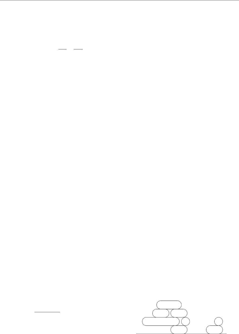
Informally, a heap is what we would imagine. We

take a collection of ‘‘pieces,’’ say B

, B

, ..., and put

them one upon the other, sometimes also sideways,

to form a ‘‘heap,’’ see Figure 6.

There, we imagine that pieces can only move

vertically, so that the heap in Figure 6 would indeed

form a stable arrangement. Note that we allow

several copies of a piece to appear in a heap. (This

means that they differ only by a vertical translation.)

For example, in Figure 6 there appear two copies of

. Under these assumptions, there are pieces which

can move past each other, and others which cannot.

For example, in Figure 6, we can move the piece B

higher up, thus moving it higher than B

if we wish.

However, we cannot move B

higher than B

Figure 6 A heap of pieces.

562 Combinatorics: Overview

because B

blocks the way. On the other hand, we

can move B

past B

(thus taking B

with us). Thus,

a rigorous way to introduce heaps is by beginning

with a set B of pieces (in our example, B=

, B

, ..., B

}), and we declare which pieces can

be moved past another and which cannot. We

indicate this by a symmetric relation R: we write

aRb to indicate that a cannot move past b (and vice

versa). When we consider a word a

...a

pieces, a

2B, we think of it as putting first a

, then

putting a

on top of it (and, possibly, moving it past

), then putting a

on top of what we already have,

etc. We declare two words to be equivalent if one

arises from the other by commuting adjacent letters

which are not in relation. A heap is then an

equivalence class of words under this equivalence

relation. What we have described just now is indeed

the original definition of Cartier and Foata.

The class of heaps which occurs most frequently

in applications is the class of heaps of monomers

and dimers, which we now introduce. Let B= M [ D,

where M= {m

, m

, ...} is the set of monomers and

D= {d

, d

, ...} is the set of dimers. We think of a

monomer m

as a point, symbolized by a circle,

with x-coordinate i,seeFigure 7.Wethink

of a dimer d

as two points, symbolized by circles,

with x-coordinates i  1andi which are connected

by an edge, see Figure 7. We impose the relations

, m

iþ1

, i = 0, 1, ..., d

, i  1 

j  i, and extend R to a symmetric relation. Figure 8

shows two heaps of momomers and dimers.

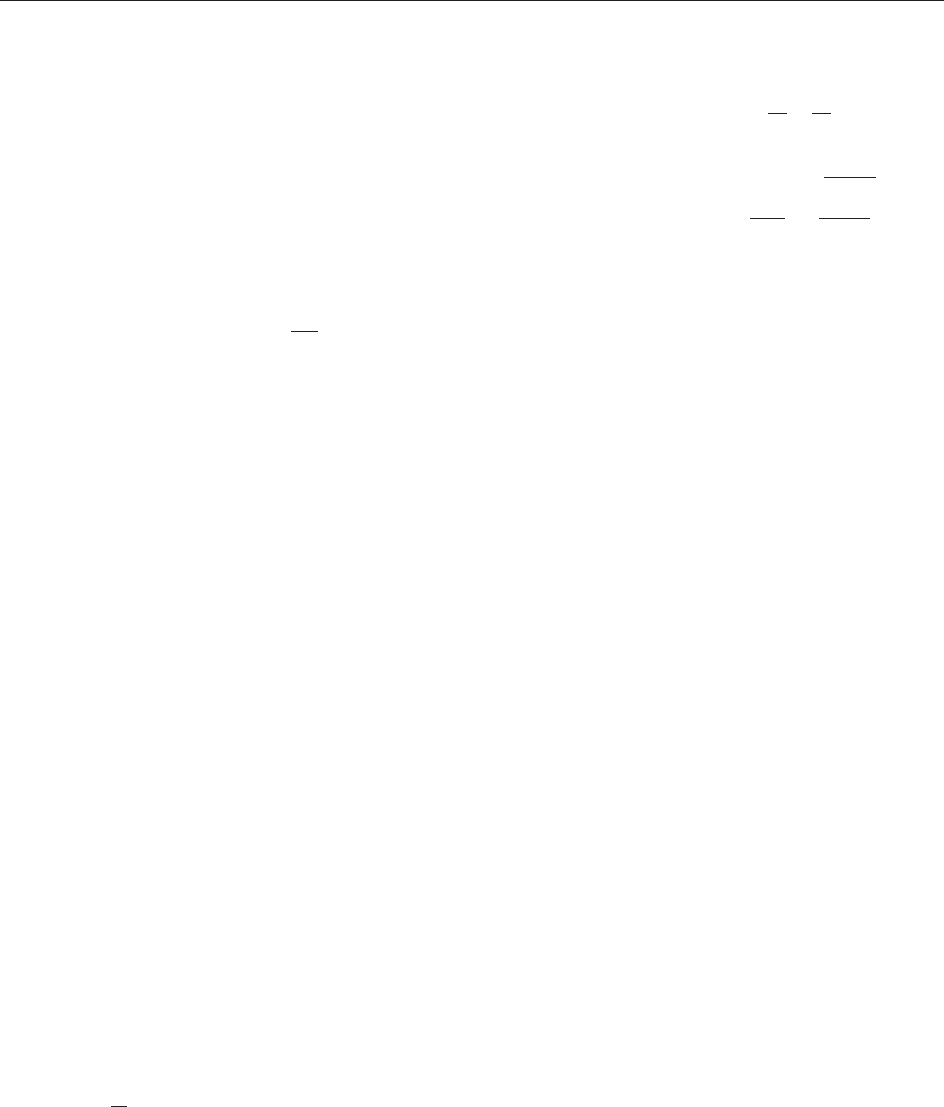
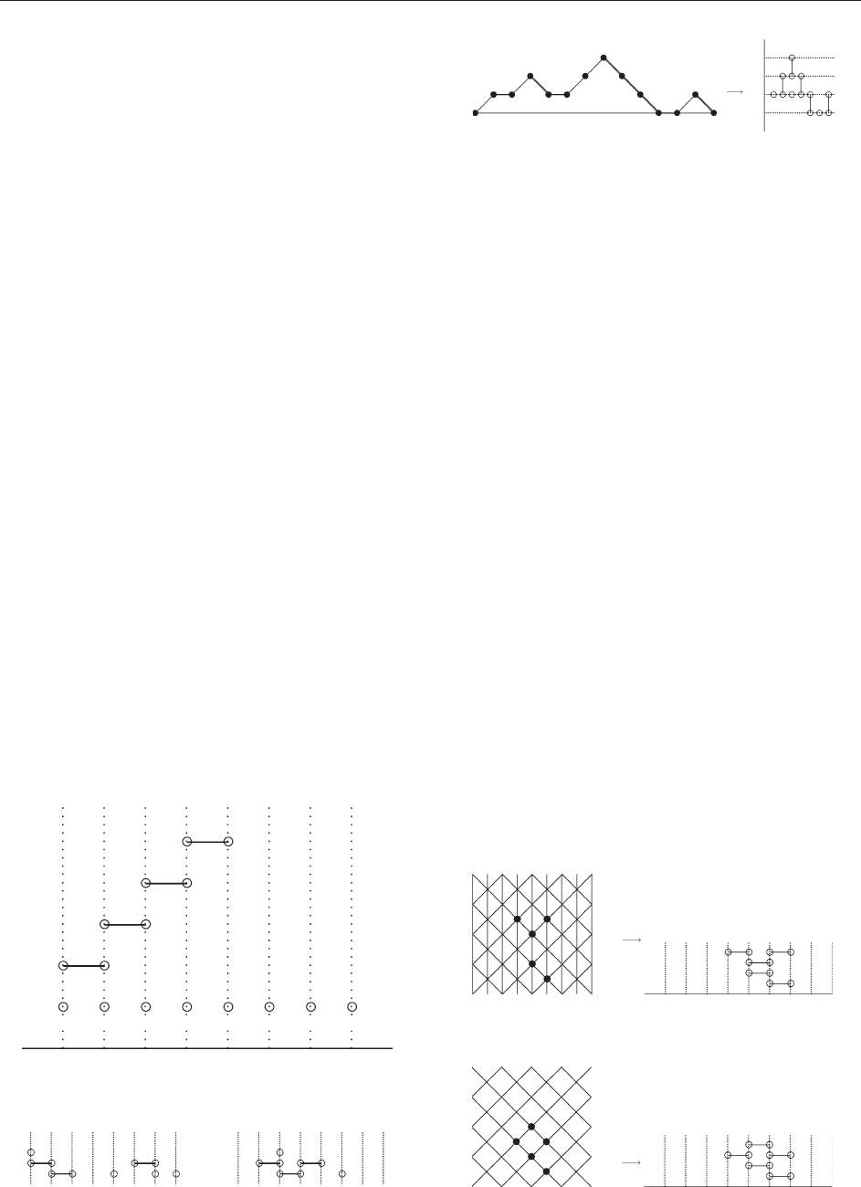
For example, Motzkin paths are in bijection with

heaps of monomers and dimers. To see this, given a

Motzkin path, we read the steps of the path from

the beginning to the end. Whenever we read a level-

step at height h, we make it into a monomer with

x-coordinate h, whenever we read a down-step from

height h to height h  1, we make it into a dimer

whose endpoints have x-coordinates h  1 and h.

Up-steps are ignored. Figure 9 shows an example. In

the figure, the heap is not in ‘‘standard’’ fashion, in

the sense that the x-axis is not shown as a horizontal

line but as a vertical line (cf. Figure 7). But it could

be easily transformed into ‘‘standard’’ fashion by a

simple reflection with respect to a line of slope 1.

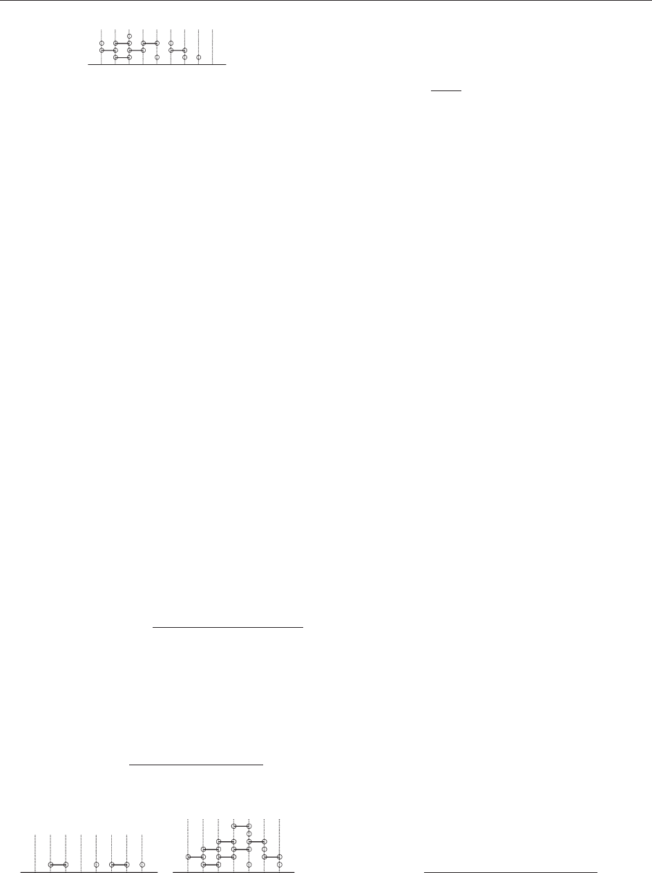
Lattice animals on the triangular lattice and on the

quadratic lattice are also in bijection with heaps, this

time with heaps consisting entirely out of dimers.

Given an animal, one simply replaces each vertex of

the animal by a dimer, see Figures 10 and 11.While

in the case of animals on the triangular lattice this

gives a constraintless bijection (see Figure 10), in the

case of the quadratic lattice this sets up a bijection

with heaps of dimers in which two dimers of the

same type can never be placed directly one over the

other (see Figure 11). For example, two dimers d

one placed directly over the other (as they occur in

Figure 10), are forbidden under this rule.

Next we make heaps into a monoid by introdu-

cing a composition of heaps. (A monoid is a set with

a binary operation which is associative.) Intuitively,

given two heaps H

and H

, the composition of H

and H

, the heap H

 H

, is the heap which results

01234567

Figure 7 Monomers and dimers.

01234567 01234567

Figure 8 Two heaps of monomers and dimers.

Figure 9 Bijection between Motzkin paths and heaps of

monomers and dimers.

012345678

Figure 10 Bijection between animals and heaps of dimers.

012345678

Figure 11 Bijection between animals and heaps of dimers.

Combinatorics: Overview 563

by putting H

on top of H

. In terms of words, the

composition of two heaps is the equivalence class of

the concatenation uw, where u is a word from the

equivalence class of H

, and w is a word from the

equivalence class of H

The composition of the two heaps in Figure 8 is

shown in Figure 12.

Given pieces B with relation R, let H(B, R) be the

set of all heaps consisting of pieces from B,

including the empty heap, the latter denoted by ;.

It is easy to see that the composition makes

(H(B , R),  ) into a monoid with unit ;.

For the statement of the main theorem in the

theory of heaps, we need two more terms. A trivial

heap is a heap consisting of pieces all of which are

pairwise unrelated. Figure 13a shows a trivial heap

consisting of monomers and dimers. A pyramid is a

heap with exactly one maximal ( = topmost) ele-

ment. Figure 13a shows a pyramid consisting of

monomers and dimers. Finally, if H is a heap, then

we write jHj for the number of pieces in H.

In applications, heaps will have weights, which are

defined by introducing a weight w(B) for each piece B

in B, and by extending the weight w to all heaps H by

letting w(H) denote the product of all weights of the

pieces in H (multiplicities of pieces included).

Let M be a subset of the pieces B. Then, the

generating function for all heaps with maximal

pieces contained in M is given by

H2HðB;RÞ

maximal pieces M

wðHÞ¼

T2T ðBnM;RÞ

ð1Þ

jTj

wðTÞ

T2T ðB;RÞ

ð1Þ

jTj

wðTÞ

½38

where T (B, R) denotes the set of all trivial heaps

with pieces from B. In particular, the generating

function for all heaps is given by

H2HðB;RÞ

wðHÞ¼

T2T ðB;RÞ

ð1Þ

jTj

wðTÞ

½39

Furthermore, if P(B , R) denotes the set of all

pyramids with pieces from B, then

P2PðB;RÞ

wðPÞ

jPj

¼ log

H2HðB;RÞ

wðHÞ

½40

where jPj is the number of pieces of P. (As the

reader will have guessed, this is a consequence of the

‘‘exponential principle’’ mentioned in the section

‘‘generatingfunctions.’’)

The Transfer Matrix Method

The transfer matrix method (cf. Stanley (1986),

chapter4forfurtherreading)applieswheneverwe

are able to build the combinatorial objects that we

are interested in by moving on a finite number of

states in a step-by-step fashion, where the current

step does not depend on the previous ones. (In

statistical language, we are considering a finite-state

Markov chain.) For example, Motzkin paths which

are constrained to stay between two parallel lines,

say between y = 0 and y = K, can be described in

such a way: the states are the heights 0, 1, ..., K,

and, if we are in state h, then in the next step we are

allowed to move to states h þ 1, h,orh  1, except

that from state 0 we cannot move to 1 (there is no

state 1), and when we are in state K we cannot

move to K þ 1 (there is no state K þ 1).

For describing the general situation, let G = (V, E)

be a directed graph with vertex set V and edge set E.Let

(u, v) denote the number of walks from vertex u to

vertex v along edges of G. To compute these numbers,

we consider the adjacency matrix of G, A(G). By

definition, using our notation, A(G) = (w

(u, v))

u, v2V

Obviously, (w

(u, v))

u, v2V

= (A(G))

.Thus,

n¼0

ðu; vÞx

u;v2V

n¼0

ðAðGÞÞ

¼ I

 AðGÞx

ðÞ

1

where I

is the n  n identity matrix. In other words,

the generating functions

n = 0

(u, v)x

for the

walk numbers between u and v form the entries of a

matrix which is the inverse matrix of I

 A(G)x.By

elementary linear algebra,

n¼0

ðu; vÞx

ð1Þ

#uþ#v

detðI

 Að GÞxÞ

v;u

detðI

 AðGÞ xÞ

½41

where det (I

 A(G)x)

v, u

is the minor of I

 A(G)x

with the row indexed by v and the column indexed

012345678

Figure 12 The composition of the heaps in Figure 8.

01234567 0123456

(a) (b)

Figure 13 (a) A trivial heap. (b) A pyramid.

564 Combinatorics: Overview